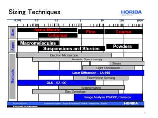
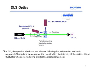
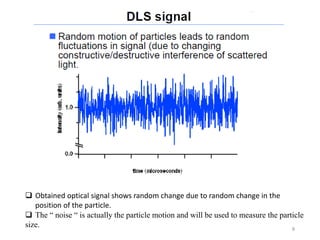
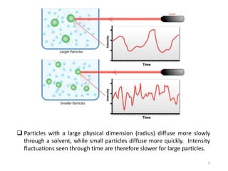
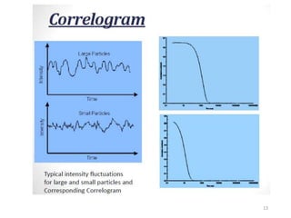
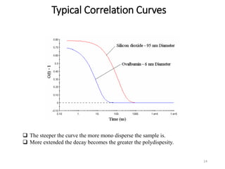
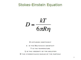
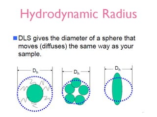
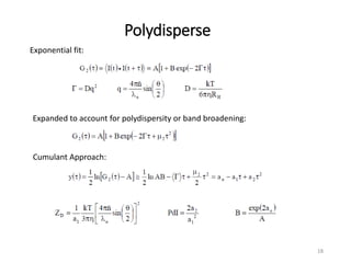
Dynamic light scattering measures the fluctuation changes in the intensity of scattered light to determine particle size and properties. It works by measuring the rate at which the intensity of scattered light fluctuates due to Brownian motion of particles. Larger particles diffuse more slowly than smaller particles, so intensity fluctuations are slower for large particles. The correlation function contains information about particle diffusion, with steeper curves indicating more monodisperse samples and more extended decay indicating greater polydispersity. Dynamic light scattering can determine particle size distribution, hydrodynamic radius, and diffusion coefficient.

1. Dynamic Light Scattering
1
Suman Kundu
Contact: sumankundu.sxc@gmail.com

2. 2
Static Light Scattering
Measures Total Intensity of Scattered Light
(Mass(M), Size (rg), Second Virial Coefficient (A2)
Dynamic Light Scattering
Measures Fluctuation Changes on The Intensity of the
Scattered light
(Diffusion Constant (DT), Size, Rh, Polydispersity Index)

3. 3
Dynamic Light Scattering
 Particle size can be determined by measuring the random change in
intensity of light scattered from suspension.
 It measure and interpolate the light scattering up to microsecond.
 So it measure real time intensity, thus measuring the dynamic
properties.
 Size distribution, Hydrodynamic radius, Diffusion coefficient

4. 4
 For measuring Hydrodynamic Size of nanoparticle, protein and biomaterial
 One can also study stability of nanoparticles as function of time
 Good for detecting the aggregation of the particles
 Required small volume of sample
 Complete recovery of sample after measurement
 Sample preparation is not required for the measurement
Application of DLS

5. 5

6. 6
 In DLS, the speed at which the particles are diffusing due to Brownian motion is
measured. This is done by measuring the rate at which the intensity of the scattered light
fluctuates when detected using a suitable optical arrangement.

7. 7
Brownian motion is the fundamental of this instrument
Brownian motion of the particle is random motion due to the
bombardment by the solvent molecule surround them.
 Brownian motion of the particles are related to size.
 It describes the way in which very small particles move in fluid
suspension
It is related to the Viscosity and Temperature.
Brownian motion

8. 8
 Obtained optical signal shows random change due to random change in the
position of the particle.
 The “ noise “ is actually the particle motion and will be used to measure the particle
size.

9. 9
 Particles with a large physical dimension (radius) diffuse more slowly
through a solvent, while small particles diffuse more quickly. Intensity
fluctuations seen through time are therefore slower for large particles.

10. 10
 A correlation function is statistical correlation between random variables at two
different points in space or time, usually as a function of the spatial or temporal
distance between the points.
 Within the correlation curve all of the information regarding the diffusion of
particles within the sample being measured.

11. 11
 A correlator is basically a signal comparator. . It is designed to measure the degree
of similarity between two signals, or one signal with itself at varying time
intervals. If the intensity at time t is compared with the intensity at time t+δt, there
will be a strong correlation between two signal.
 Correlation of a signal arriving from random source will decrease with time.
 If the particle will large the signal will changes slowly and correlation will sustain
for long time.
How does a Correlator Work

12. Measure Timescale of Diffusion:
Autocorrelation Function
12

13. 13

14. 14
Typical Correlation Curves
 The steeper the curve the more mono disperse the sample is.
 More extended the decay becomes the greater the polydispesity.

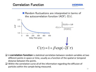
15. The Correlation Function for monodisperse particle
15
G() = A [ 1 + B exp (-2)]
A = the baseline of the correlation function
B = intercept of the correlation function.
 = Dq2
D = translational diffusion coefficient, q = scattering vector
q = (4 n / o) sin (/2)
n = refractive index of dispersant
o = wavelength of the laser
 = scattering angle.

16. 16

17. 17

18. Polydisperse
18
Exponential fit:
Expanded to account for polydispersity or band broadening:
Cumulant Approach:

19. Analysis
19

20. Polydispersity Index
• 0 to 0.05 - Monodisperse
• 0.05 to 0.08 - Nearly Monodisperse
• 0.08 to 0.7 - Mid Range Polydispersity
• Greater than 0.7 – Very Polydisperse; Probably not
suited for DLS Measurements
20

21. Intensity Size distributions
21

22. Typical Results
22

23. 23

24. 24

25. 25
Thank You