Presentation by Martijn Visser and Huite Bootsma (Deltares) at the iMOD International User Day 2018, during Delft Software Days - Edition 2018. Tuesday 13 November 2018, Delft.

1. Work with iMOD MODFLOW models in Python
Martijn Visser, martijn.visser@deltares.nl
Huite Bootsma, huite.bootsma@deltares.nl
November 16, 2018
Note: this document has been translated from a Jupyter Notebook. The content will also be made avail-
able in Jupyter Notebook form here:
https://gitlab.com/deltares/imod-python/tree/master/examples
1 Introduction
Python has seen very strong growth in recent years:
https://stackoverflow.blog/2017/09/06/incredible-growth-python/
1

2. https://stackoverflow.blog/2017/09/14/python-growing-quickly/
Technical computing is an important driver of this growth: django and flask are web devel-
opment frameworks and show moderate growth; pandas, numpy, and matplotlib are packages
typically used for technical computing and show very strong growth.
2

3. 1.1 pip install imod
The python imod package is available on PyPI.org and can be installed with pip install imod.
PyPI page: https://pypi.org/project/imod/
Source code is available here: https://gitlab.com/deltares/imod-python
Documentation can be found here: https://deltares.gitlab.io/imod-python/
The package is built on xarray and pandas:
• pandas makes working with tabular data easy, for example timeseries
• xarray makes working with N-D arrays easy, for example groundwater heads that
vary over (x, y, time, and layer). It’s effectively an in-memory netCDF file.
• imod Python package makes working with iMODFLOW models in Python easy
3

4. 1.2 What’s so great about pandas?
In [1]: import pandas
import matplotlib.pyplot as plt
%matplotlib inline
In [2]: fig = plt.figure(figsize=(25, 10))
df = pandas.read_csv("groundwater_timeseries.csv", index_col=1, parse_dates=[1])
df["head"].plot()
df["head"].rolling(window=180, center=True).mean().plot()
Out[2]: <matplotlib.axes._subplots.AxesSubplot at 0x8d20f60>
1.2.1 xarray versus numpy
# numpy style
>>> array[[0, 1, 3], :, :].max(axis=2)
# xarray style
>>> ds.sel(time="2017-11-28").max(dim="station")
4

5. 2 Convert Excel to IPF
In [3]: import pandas
import imod
In [4]: df = pandas.read_excel("geophysical_measurements.xlsx")
In [6]: df.head()
Out[6]: CPT_name Depth_m Depth_m_NAP Sonic_velocity_m/sec Xcoord Ycoord
0 1210032_02 5.00 -3.74 1883.321 249255 607899
1 1210032_02 5.00 -3.74 1883.321 249255 607899
2 1210032_02 5.02 -3.76 1885.021 249255 607899
3 1210032_02 5.02 -3.76 1885.021 249255 607899
4 1210032_02 5.04 -3.78 1886.720 249255 607899
In [7]: df = df.rename(columns={"CPT_name": "id",
"Depth_m_NAP": "top",
"Xcoord": "x",
"Ycoord": "y"})
In [8]: imod.ipf.save("ipf_data/geophysical_measurements.ipf", df, itype="cpt")
5

6. 3 Let’s build a model from scratch!
3.1 After:
• Toth, 1963, A Theoretical Analysis of Groundwater Flow in Small Drainage Basins
• Xiao-Wei Jiang, Li Wan, Xu-Sheng Wang, Shemin Ge, and Jie Liu, 2008, Effect of exponential
decay in hydraulic conductivity with depth on regional groundwater flow
The goal is to simulate an aquifer with a sloping phreatic water table, with local drainage:
Which results in a region flow, with nested systems:
6

7. In [9]: from collections import OrderedDict
import subprocess
import imod
import matplotlib.pyplot as plt
import numpy as np
import xarray as xr
%matplotlib inline
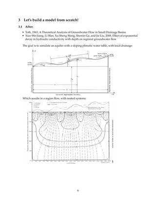
The phreatic water table is given by the following function (Toth, 1963):
zx(x) = z0 + x tan α + a
cos(α)
sin( bx
cos α )
Conductivity decreases exponentially with depth (Jiang et al., 2009):
k(z) = k0 exp[−A(zs − z)]
We can translate these functions into Python as follows:
In [10]: def phreatic_head(z0, x, a, alpha, b):
"""Synthetic ground surface, a la Toth 1963"""
return (z0 + x * np.tan(alpha) + a / np.cos(alpha)
* np.sin((b * x) / (np.cos(alpha))))
def conductivity(k0, z, A):
"""Exponentially decaying conductivity"""
return k0 * np.exp(-A * (1000.0 - z))
7

8. 4 Generate the phreatic boundary condition
In [11]: z0 = 1000.0
x = np.arange(0.0, 6000.0, 10.0) + 5.0
a = 15.0
b = np.pi / 750.0
alpha = 0.02
In [12]: head_top = xr.DataArray(
data=phreatic_head(z0, x, a, alpha, b),
coords={"x": x},
dims=("x")
)
In [13]: fig = plt.figure(figsize=(10, 5))
head_top.plot()
Out[13]: [<matplotlib.lines.Line2D at 0xbc34d68>]
8

9. 5 Generate conductivity
In [14]: ncol = x.size
nrow = 1
nlay = 100
coords = {"layer": np.arange(1, 101), "y": [5.0], "x": x}
dims = ("layer", "y", "x")
bnd = xr.DataArray(
data=np.full((nlay, nrow, ncol), 1.0),
coords=coords,
dims=dims,
)
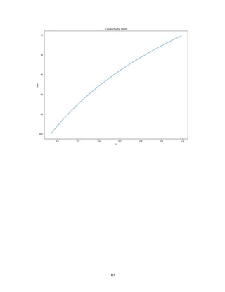
In [15]: k0 = 1.0 # m/d
A = 0.001
z = np.arange(0.0, 1000.0, 10.0) + 5.0
k_z = xr.DataArray(
data=conductivity(k0, z, A),
coords={"z": z},
dims=("z"),
)
k_z.coords["z"] = bnd.coords["layer"].values[::-1]
k_z = k_z.rename({"z": "layer"})
kh = bnd.copy() * k_z
In [16]: fig = plt.figure(figsize=(13, 10))
k_z.plot(y="layer")
plt.title("Conductivity (m/d)")
plt.gca().invert_yaxis()
plt.xlabel("x")
Out[16]: Text(0.5,0,'x')
9

10. 10

11. 6 Generate the iMODFLOW model files
In [17]: model = OrderedDict()
model["bnd"] = bnd
# constant head in the first layer
model["bnd"].sel(layer=1)[...] = -1.0
model["kdw"] = kh * 10.0
model["vcw"] = 10.0 / kh
model["shd"] = bnd * head_top
# We have to an additional package for it to run...
model["rch"] = xr.full_like(bnd.sel(layer=1), 0.0)
In [18]: imod.write("toth", model)
Now let’s inspect these files, and run the model.
11

12. 6.1 Load the results
In [19]: head = imod.idf.load("results/head/*.idf")
head
Out[19]: <xarray.DataArray 'head' (layer: 100, y: 1, x: 600)>
dask.array<shape=(100, 1, 600), dtype=float32, chunksize=(1, 1, 600)>
Coordinates:
* y (y) float64 5.0
* x (x) float64 5.0 15.0 25.0 35.0 ... 5.975e+03 5.985e+03 5.995e+03
* layer (layer) int32 1 2 3 4 5 6 7 8 9 10 ... 92 93 94 95 96 97 98 99 100
Attributes:
res: (10.0, 10.0)
transform: (10.0, 0.0, 0.0, 0.0, -10.0, 10.0)
In [20]: fig = plt.figure(figsize=(10, 6))
head.isel(y=0).plot()
plt.gca().invert_yaxis()
12

13. 7 Look at streamlines
In [21]: vz = imod.idf.load("results/bdgflf/*.idf").isel(y=0).values[:]
vx = imod.idf.load("results/bdgfrf/*.idf").isel(y=0).values[:]
In [22]: f, (ax1, ax2) = plt.subplots(ncols=1, nrows=2, sharex=True,
gridspec_kw={'height_ratios': [0.2, 0.8]},
figsize=(15, 5)
)
ax1.plot(head_top["x"], head_top.values, color="k")
ax1.set_ylabel("head(m)", size=16)
ax2.streamplot(x, z[:], vx, vz, arrowsize=2)
ax2.invert_yaxis()
ax2.set_ylabel("layer", size=16)
ax2.set_xlabel("x", size=16)
f.set_figheight(10.0)
13