The document provides various examples of using R programming for basic calculus, including functions for plotting, differentiation, integration, and solving equations. It includes commands for creating functions, plotting data, modeling relationships, and applying statistical methods. The use of the 'mosaic' and 'manipulate' libraries is demonstrated through practical examples for educational purposes.

1. Prepared by VOLKAN OBAN
Basic Calculus in R.
install.packages("mosaic")
library(mosaic)
Example:
> f <- makeFun(m * x + b ~ x, m = 3.5, b = 10)
>
> f(x = 2)
[1] 17
>
> g <- makeFun(A * x * cos(pi * x * y) ~ x + y, A = 3)
> g
function (x, y, A = 3)
A * x * cos(pi * x * y)
>
> g(x = 1, y = 2)
[1] 3
> > plotFun(A * exp(k * t) * sin(2 * pi * t/P) ~ t + k, t.lim = range(0, 1
0), k.lim = range(-0.3,
+
0), A = 10, P = 4)

2. Example
Example:
> library(manipulate)
> plotFun(A * exp(k * t) * sin(2 * pi * t/P) ~ t + k, t.lim = range(0, 10),
k.lim = range(-0.3,
+
0), A = 10, P = 4, surface = TRUE)

4. Example:
> plotFun(dt(t, df) ~ t + df, t.lim = range(-3, 3), df.lim = range(1, 10))
Derivative:
>library(mosaic)
> D(sin(x) ~ x)
function (x)
cos(x)
> D(A * x^2 * sin(y) ~ x)
function (x, A, y)
A * (2 * x) * sin(y)
> D(A * x^2 * sin(y) ~ x + y)
function (x, y, A)
A * (2 * x) * cos(y)

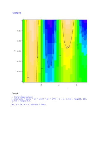
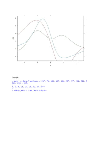
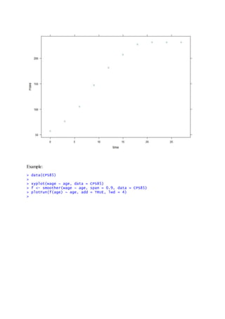
5. Example:
> F = antiD(a * x^2 ~ x, a = 1)
> F
function (x, a = 1, C = 0)
a * 1/3 * x^3 + C
> F = antiD(dnorm(x, mean = 6000, sd = 0.01) ~ x, lower.bound = 6000)
> F(Inf) - F(-Inf)
[1] 1
>
Solving..
findZeros(sin(t) ~ t, t.lim = range(-5, 1))
> findZeros(sin(t) ~ t, t.lim = range(-5, 1))
t
1 -6.2832
2 -3.1416
3 0.0000
4 3.1416
Example:
> solve(4 * sin(3 * x) == 2 ~ x, near = 0, within = 1)
x
1 0.1746
2 0.8726
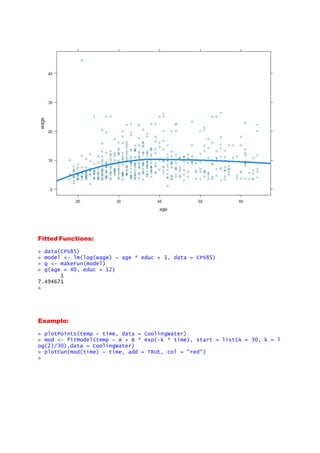
Example:
> f <- rfun(~x, seed = 345)
> g <- rfun(~x)
> h <- rfun(~x)
> plotFun(f(x) ~ x, x.lim = range(-5, 5))
> plotFun(g(x) ~ x, add = TRUE, col = "red")
> plotFun(h(x) ~ x, add = TRUE, col = "darkgreen")
>

6. Example:
> Water <- data.frame(mass = c(57, 76, 105, 147, 181, 207, 227, 231, 231, 2
31), time = c(0,
+
3, 6, 9, 12, 15, 18, 21, 24, 27))
>
> xyplot(mass ~ time, data = Water)

7. Example:
> data(CPS85)
>
> xyplot(wage ~ age, data = CPS85)
> f <- smoother(wage ~ age, span = 0.9, data = CPS85)
> plotFun(f(age) ~ age, add = TRUE, lwd = 4)
>

8. Fitted Functions:
> data(CPS85)
> model <- lm(log(wage) ~ age * educ + 1, data = CPS85)
> g <- makeFun(model)
> g(age = 40, educ = 12)
1
7.494671
>
Example:
> plotPoints(temp ~ time, data = CoolingWater)
> mod <- fitModel(temp ~ A + B * exp(-k * time), start = list(A = 30, k = l
og(2)/30),data = CoolingWater)
> plotFun(mod(time) ~ time, add = TRUE, col = "red")
>

9. Mixed Examples:
1
> f = function(x){ x^2 + 2*x }
>
> f(pi)
[1] 16.15279
2-
> findZeros( sin(x)-0.35 ~ x, x.lim=range(-20,20) )
x
1 -12.2088
2 -9.7823
3 -5.9256
4 -3.4991
5 0.3576
6 2.7840
7 6.6407
8 9.0672
9 12.9239
10 15.3504
3-
> findZeros(sin(x^2)*(cos(sqrt(x^4+3)-x^2))-x+1~x,x.lim=range(1,2))
x
1 1.5576
4-
> f3 = makeFun( sin(x^2) - 100~x)
> f3(x=2)
[1] -100.7568

10. 5-
> F = antiD( exp(x^2) ~ x )
> F(x=2) - F(x=-1)
[1] 17.91528
6-Dif.Eq.
> soln <- integrateODE( dx ~ r*x*(1-x/K),x=1, K=10, r=.5, tdur=list(from=0,
to=20))
> soln$x(0:5)
[1] 1.000000 1.548281 2.319693 3.324279 4.508531 5.751209
7-
> plotFun( exp(-t/10)*sin(2*pi*x/5) ~ x&t,x.lim=range(0,5), t.lim=range(0,1
0) )
8-
> newF = antiD(exp(x)*x^2 ~ x, x.from=1)
> F(x=2) #default lower bound is 0
[1] 16.45263