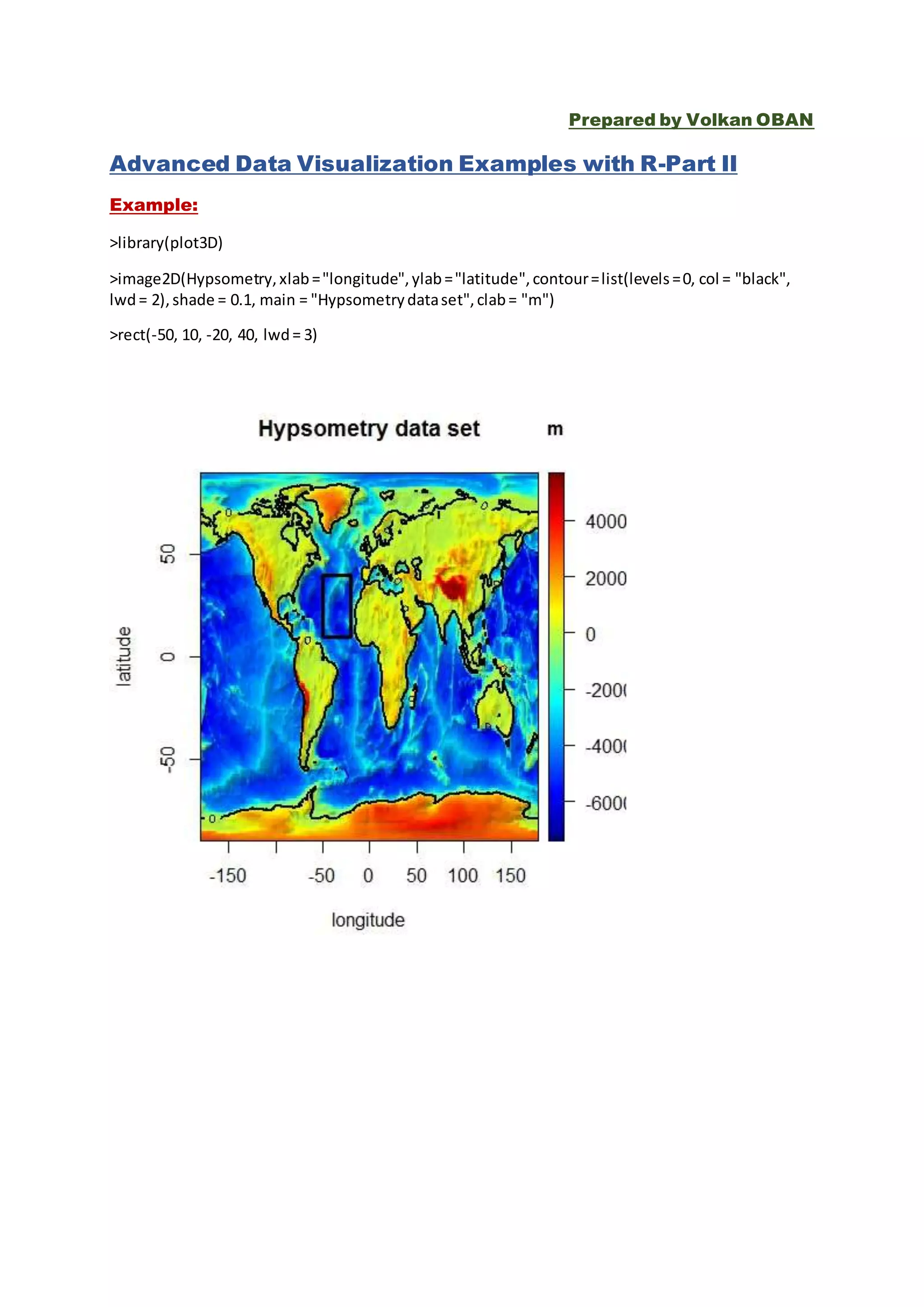
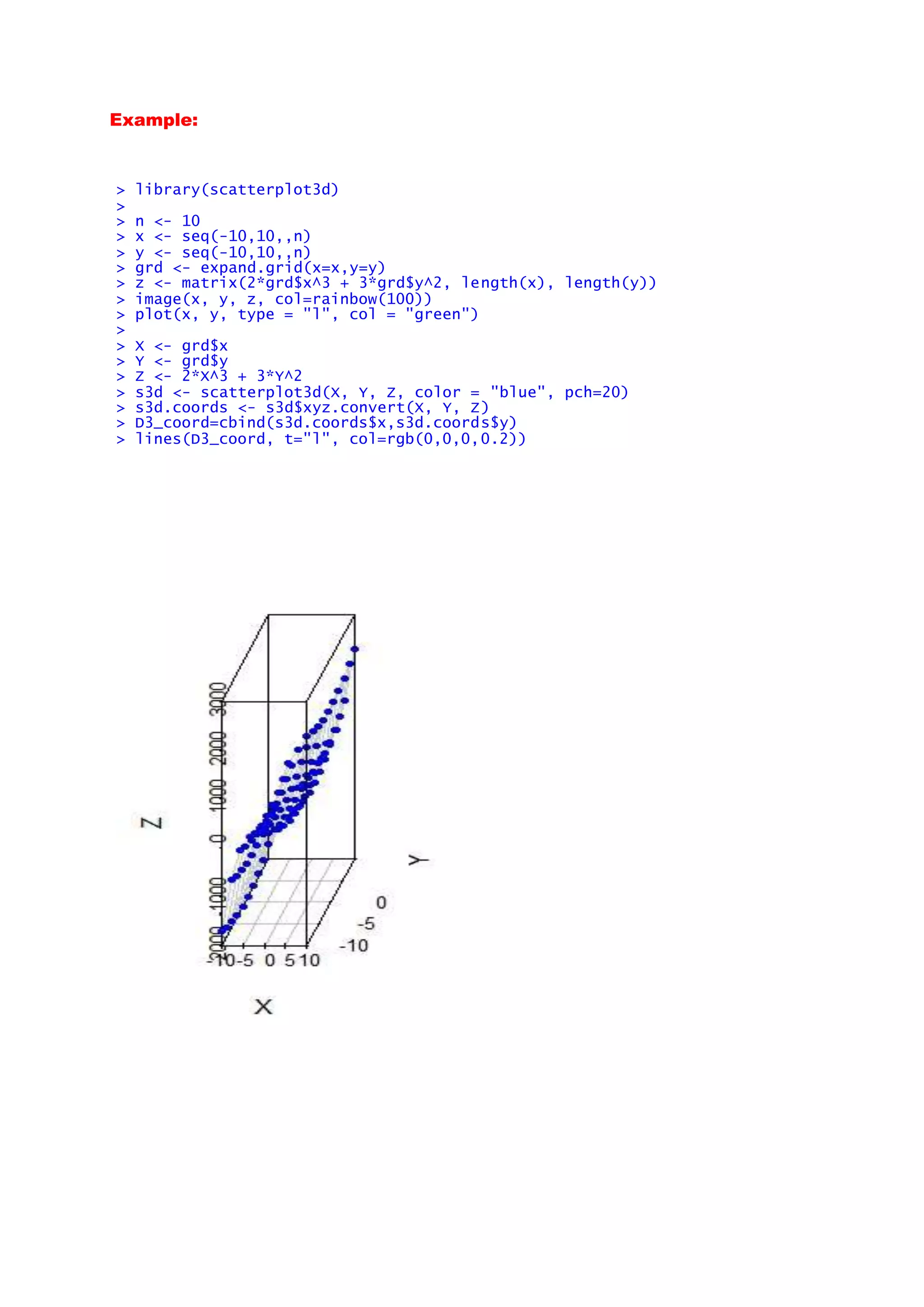
Prepared by Volkan OBAN
Advanced Data Visualization Examples with R-Part II
Example:
>library(plot3D)
>image2D(Hypsometry,xlab="longitude",ylab="latitude",contour=list(levels=0, col = "black",
lwd= 2),shade = 0.1, main = "Hypsometrydataset",clab= "m")
>rect(-50, 10, -20, 40, lwd= 3)
Example:
>library(plot3D)
> par(mfrow = c(2, 2), mar = c(0, 0, 0, 0))
> # Shape 1
> M <- mesh(seq(0, 6*pi, length.out = 80),
+ seq(pi/3, pi, length.out = 80))
> u <- M$x ; v <- M$y
> x <- u/2 * sin(v) * cos(u)
> y <- u/2 * sin(v) * sin(u)
> z <- u/2 * cos(v)
> surf3D(x, y, z, colvar = z, colkey = FALSE, box = FALSE)
> # Shape 2: add border
> M <- mesh(seq(0, 2*pi, length.out = 80),
+ seq(0, 2*pi, length.out = 80))
> u <- M$x ; v <- M$y
> x <- sin(u)
> y <- sin(v)
> z <- sin(u + v)
> surf3D(x, y, z, colvar = z, border = "black", colkey = FALSE)
> # shape 3: uses same mesh, white facets
> x <- (3 + cos(v/2)*sin(u) - sin(v/2)*sin(2*u))*cos(v)
> y <- (3 + cos(v/2)*sin(u) - sin(v/2)*sin(2*u))*sin(v)
Example:
> par (mfrow = c(1, 2))
> arrows2D(x0 = runif(10), y0 = runif(10),
+ x1 = runif(10), y1 = runif(10), colvar = 1:10,
+ code = 3, main = "arrows2D")
> arrows3D(x0 = runif(10), y0 = runif(10), z0 = runif(10),
+ x1 = runif(10), y1 = runif(10), z1 = runif(10),
+ colvar = 1:10, code = 1:3, main = "arrows3D", colkey = FALSE)
>
Example:
> persp3D(z = volcano, zlim = c(-60, 200), phi = 20,
colkey = list(length = 0.2, width = 0.4, shift = 0.15,
cex.axis = 0.8, cex.clab = 0.85), lighting = TRUE, lphi = 90,clab = c("","
height","m"), bty = "f", plot = FALSE)
> # create gradient in x-direction
> Vx <- volcano[-1, ] - volcano[-nrow(volcano), ]
> # add as image with own color key, at bottom
> image3D(z = -60, colvar = Vx/10, add = TRUE,colkey = list(length = 0.2,
width = 0.4, shift = -0.15,cex.axis = 0.8, cex.clab = 0.85),clab = c("","g
radient","m/m"), plot = FALSE)
> # add contour
> contour3D(z = -60+0.01, colvar = Vx/10, add = TRUE,col = "black", plot =
TRUE)
Example:
> library(scatterplot3d)
>
> n <- 10
> x <- seq(-10,10,,n)
> y <- seq(-10,10,,n)
> grd <- expand.grid(x=x,y=y)
> z <- matrix(2*grd$x^3 + 3*grd$y^2, length(x), length(y))
> image(x, y, z, col=rainbow(100))
> plot(x, y, type = "l", col = "green")
>
> X <- grd$x
> Y <- grd$y
> Z <- 2*X^3 + 3*Y^2
> s3d <- scatterplot3d(X, Y, Z, color = "blue", pch=20)
> s3d.coords <- s3d$xyz.convert(X, Y, Z)
> D3_coord=cbind(s3d.coords$x,s3d.coords$y)
> lines(D3_coord, t="l", col=rgb(0,0,0,0.2))
Example:
 barplot(matrix(sample(1:4, 16, replace=T),ncol=4),angle=45, de
nsity=1:4*10, col=1)
Example:
require(plot3D)
lon <- seq(165.5, 188.5, length.out = 30)
lat <- seq(-38.5, -10, length.out = 30)
xy <- table(cut(quakes$long, lon),
cut(quakes$lat, lat))
xmid <- 0.5*(lon[-1] + lon[-length(lon)])
ymid <- 0.5*(lat[-1] + lat[-length(lat)])
par (mar = par("mar") + c(0, 0, 0, 2))
hist3D(x = xmid, y = ymid, z = xy,
zlim = c(-20, 40), main = "Earth quakes",
ylab = "latitude", xlab = "longitude",
zlab = "counts", bty= "g", phi = 5, theta = 25,
shade = 0.2, col = "white", border = "black",
d = 1, ticktype = "detailed")
with (quakes, scatter3D(x = long, y = lat,
z = rep(-20, length.out = length(long)),
colvar = quakes$depth, col = gg.col(100),
add = TRUE, pch = 18, clab = c("depth", "m"),
colkey = list(length = 0.5, width = 0.5,
dist = 0.05, cex.axis = 0.8, cex.clab = 0.8)))
Example:
> library(maps)
> coplot(lat ~ long | depth, data = quakes, number=4,
panel=function(x, y, ...) {
usr <- par("usr")
rect(usr[1], usr[3], usr[2], usr[4], col="white")
map("world2", regions=c("New Zealand", "Fiji"),
add=TRUE, lwd=0.1, fill=TRUE, col="grey")
text(180, -13, "Fiji", adj=1, cex=0.7)
text(170, -35, "NZ", cex=0.7)
points(x, y, pch=".") })
Example:
> library(grid)
> levels <- round(seq(90, 10, length=25))
> greys <- paste("grey", c(levels, rev(levels)), sep="")
> grid.circle(x=seq(0.1, 0.9, length=100),y=0.5 + 0.4*sin(seq(0, 2*pi, leng
th=100)), r=abs(0.1*cos(seq(0, 2*pi, length=100))),gp=gpar(col=greys))
Example:
> library(misc3d)
> x <- seq(-2,2,len=50)
> g <- expand.grid(x = x, y = x, z = x)
> v <- array(g$x^4 + g$y^4 + g$z^4, rep(length(x),3))
> con <- computeContour3d(v, max(v), 1)
> drawScene(makeTriangles(con))
misc3d: Miscellaneous 3D Plots
Example:
> library(misc3d)
> f <- function(x, y, z)x^2+y^2+z^2
> x <- seq(-2,2,len=20)
> contour3d(f,4,x,x,x)
> contour3d(f,4,x,x,x, engine = "standard")
> # ball with one corner removed.
> contour3d(f,4,x,x,x, mask = function(x,y,z) x > 0 | y > 0 | z > 0)
> contour3d(f,4,x,x,x, mask = function(x,y,z) x > 0 | y > 0 | z > 0,
engine="standard", screen = list(x = 290, y = -20),color = "red", color2 =
"white")
Example:
> library(AnalyzeFMRI)
Zorunlu paket yükleniyor: tcltk
Zorunlu paket yükleniyor: R.matlab
R.matlab v3.6.0 (2016-07-05) successfully loaded. See ?R.matlab for help
> a <- f.read.analyze.volume(system.file("example.img", package="AnalyzeFMR
I"))
> a <- a[,,,1]
> contour3d(a, 1:64, 1:64, 1.5*(1:21), lev=c(3000, 8000, 10000),
+ alpha = c(0.2, 0.5, 1), color = c("white", "red", "green"))
> # alternative masking out a corner
> m <- array(TRUE, dim(a))
> m[1:30,1:30,1:10] <- FALSE
> contour3d(a, 1:64, 1:64, 1.5*(1:21), lev=c(3000, 8000, 10000),
+ mask = m, color = c("white", "red", "green"))
> contour3d(a, 1:64, 1:64, 1.5*(1:21), lev=c(3000, 8000, 10000),
+ color = c("white", "red", "green"),
+ color2 = c("gray", "red", "green"),
+ mask = m, engine="standard",
+ scale = FALSE, screen=list(z = 60, x = -120))
Example:
> nmix3 <- function(x, y, z, m, s) {
0.3*dnorm(x, -m, s) * dnorm(y, -m, s) * dnorm(z, -m, s) +
0.3*dnorm(x, -2*m, s) * dnorm(y, -2*m, s) * dnorm(z, -2*m, s) +
0.4*dnorm(x, -3*m, s) * dnorm(y, -3 * m, s) * dnorm(z, -3*m, s) }
> f <- function(x,y,z) nmix3(x,y,z,0.5,.1)
> n <- 20
> x <- y <- z <- seq(-2, 2, len=n)
> contour3dObj <- contour3d(f, 0.35, x, y, z, draw=FALSE, separate=TRUE)
> for(i in 1:length(contour3dObj))
contour3dObj[[i]]$color <- rainbow(length(contour3dObj))[i]
> drawScene.rgl(contour3dObj)
>
Example:
> nmix3 <- function(x, y, z, m, s) {
+ 0.4 * dnorm(x, m, s) * dnorm(y, m, s) * dnorm(z, m, s) +
+ 0.3 * dnorm(x, -m, s) * dnorm(y, -m, s) * dnorm(z, -m, s) +
+ 0.3 * dnorm(x, m, s) * dnorm(y, -1.5 * m, s) * dnorm(z, m, s)
+ }
> x<-seq(-2, 2, len=40)
> g<-expand.grid(x = x, y = x, z = x)
> v<-array(nmix3(g$x,g$y,g$z, .5,.5), c(40,40,40))
> slices3d(vol1=v, main="View of a mixture of three tri-variate normals", c
ol1=heat.colors(256))
Example:
library(ggplot2)
g <- ggplot(mtcars, aes(x=factor(cyl)))
g + geom_bar(fill = "pink",color="violet",size=2,width=.5)+ coord_flip()
Example:
>library(ggplot2)
> data("Orange")
> qplot(age, circumference, data = Orange, geom = c("point", "line"), color
= Tree)
Example:
library(plyr)
mean.prop.sw <- c(0.7, 0.6, 0.67, 0.5, 0.45, 0.48, 0.41, 0.34, 0.5, 0.33)
sd.prop.sw <- c(0.3, 0.4, 0.2, 0.35, 0.28, 0.31, 0.29, 0.26, 0.21, 0.23)
N <- 100
b <- barplot(mean.prop.sw, las = 1, xlab = " ", ylab = " ", col = "grey", c
ex.lab = 1.7,
cex.main = 1.5, axes = FALSE, ylim = c(0, 1))
axis(1, c(0.8, 2, 3.2, 4.4, 5.6, 6.8, 8, 9.2, 10.4, 11.6), 1:10, cex.axis =
1.3)
axis(2, seq(0, 0.8, by = 0.2), cex.axis = 1.3, las = 1)
mtext("Block", side = 1, line = 2.5, cex = 1.5, font = 2)
mtext("Proportion of Switches", side = 2, line = 3, cex = 1.5, font = 2)
l_ply(seq_along(b), function(x) arrows(x0 = b[x], y0 = mean.prop.sw[x], x1
= b[x],
y1 = mean.prop.sw[x] + 1.96 * sd.prop.sw[x]/sqrt(N), code = 2, length =
0.1,
angle = 90, lwd = 1.5))
Example:
>library("psych")
> library("qgraph")
>
> # Load BFI data:
> data(bfi)
> bfi <- bfi[, 1:25]
>
> # Groups and names object (not needed really, but make the plots easier t
o
> # interpret):
> Names <- scan("http://sachaepskamp.com/files/BFIitems.txt", what = "chara
cter", sep = "n")
Read 25 items
>
> # Create groups object:
> Groups <- rep(c("A", "C", "E", "N", "O"), each = 5)
>
> # Compute correlations:
> cor_bfi <- cor_auto(bfi)
Variables detected as ordinal: A1; A2; A3; A4; A5; C1; C2; C3; C4; C5; E1;
E2; E3; E4; E5; N1; N2; N3; N4; N5; O1; O2; O3; O4; O5
>
> # Plot correlation network:
> graph_cor <- qgraph(cor_bfi, layout = "spring", nodeNames = Names, groups
= Groups, legend.cex = 0.6,
+ DoNotPlot = TRUE)
>
> # Plot partial correlation network:
> graph_pcor <- qgraph(cor_bfi, graph = "concentration", layout = "spring",
nodeNames = Names,
+ groups = Groups, legend.cex = 0.6, DoNotPlot = TRUE)
>
> # Plot glasso network:
> graph_glas <- qgraph(cor_bfi, graph = "glasso", sampleSize = nrow(bfi), l
ayout = "spring",
+ nodeNames = Names, legend.cex = 0.6, groups = Groups
, legend.cex = 0.7, GLratio = 2)
Example:
> library (ggplot2)
> g <- ggplot(diamonds, aes(x = carat, y = price))
> g + geom_point(aes(color = color)) + facet_grid(cut ~ clarity)
Example:
> data("diamonds")
> ggplot(diamonds, aes(y = carat, x = cut)) + geom_violin()
Example:
> library(ggtree)
> set.seed(2015-12-31)
> tr <- rtree(15)
> p <- ggtree(tr)
>
> a <- runif(14, 0, 0.33)
> b <- runif(14, 0, 0.33)
> c <- runif(14, 0, 0.33)
> d <- 1 - a - b - c
> dat <- data.frame(a=a, b=b, c=c, d=d)
> ## input data should have a column of `node` that store the node number
> dat$node <- 15+1:14
>
> ## cols parameter indicate which columns store stats (a, b, c and d in th
is example)
> bars <- nodebar(dat, cols=1:4)
>
> inset(p, bars)
Example:
> cat("nheight weight healthn1 0.6008 0.3355 1.280n2 0.9440 0.6890 1
.208n3 0.6150 0.6980 1.036n4 1.2340 0.7617 1.395n5 0.7870 0.8910 0
.912n6 0.9150 0.9330 1.175n7 1.0490 0.9430 1.237n8 1.1840 1.0060 1
.048n9 0.7370 1.0200 1.003n10 1.0770 1.2150 0.943n11 1.1280 1.2230 0
.912n12 1.5000 1.2360 1.311n13 1.5310 1.3530 1.411n14 1.1500 1.3770 0
.603n15 1.9340 2.0734 1.073 ",
+ file = "height_weight.dat")
>
> hw <- read.table("height_weight.dat", header = T)
>
> head(hw)
height weight health
1 0.6008 0.3355 1.280
2 0.9440 0.6890 1.208
3 0.6150 0.6980 1.036
4 1.2340 0.7617 1.395
5 0.7870 0.8910 0.912
6 0.9150 0.9330 1.175
> qplot(x = weight, y = health, data = hw) + geom_smooth(method = lm)
Advanced Data Visualization Examples with R-Part II

Advanced Data Visualization Examples with R-Part II

  • 1.
    Prepared by VolkanOBAN Advanced Data Visualization Examples with R-Part II Example: >library(plot3D) >image2D(Hypsometry,xlab="longitude",ylab="latitude",contour=list(levels=0, col = "black", lwd= 2),shade = 0.1, main = "Hypsometrydataset",clab= "m") >rect(-50, 10, -20, 40, lwd= 3)
  • 2.
    Example: >library(plot3D) > par(mfrow =c(2, 2), mar = c(0, 0, 0, 0)) > # Shape 1 > M <- mesh(seq(0, 6*pi, length.out = 80), + seq(pi/3, pi, length.out = 80)) > u <- M$x ; v <- M$y > x <- u/2 * sin(v) * cos(u) > y <- u/2 * sin(v) * sin(u) > z <- u/2 * cos(v) > surf3D(x, y, z, colvar = z, colkey = FALSE, box = FALSE) > # Shape 2: add border > M <- mesh(seq(0, 2*pi, length.out = 80), + seq(0, 2*pi, length.out = 80)) > u <- M$x ; v <- M$y > x <- sin(u) > y <- sin(v) > z <- sin(u + v) > surf3D(x, y, z, colvar = z, border = "black", colkey = FALSE) > # shape 3: uses same mesh, white facets > x <- (3 + cos(v/2)*sin(u) - sin(v/2)*sin(2*u))*cos(v) > y <- (3 + cos(v/2)*sin(u) - sin(v/2)*sin(2*u))*sin(v)
  • 3.
    Example: > par (mfrow= c(1, 2)) > arrows2D(x0 = runif(10), y0 = runif(10), + x1 = runif(10), y1 = runif(10), colvar = 1:10, + code = 3, main = "arrows2D") > arrows3D(x0 = runif(10), y0 = runif(10), z0 = runif(10), + x1 = runif(10), y1 = runif(10), z1 = runif(10), + colvar = 1:10, code = 1:3, main = "arrows3D", colkey = FALSE) >
  • 4.
    Example: > persp3D(z =volcano, zlim = c(-60, 200), phi = 20, colkey = list(length = 0.2, width = 0.4, shift = 0.15, cex.axis = 0.8, cex.clab = 0.85), lighting = TRUE, lphi = 90,clab = c(""," height","m"), bty = "f", plot = FALSE) > # create gradient in x-direction > Vx <- volcano[-1, ] - volcano[-nrow(volcano), ] > # add as image with own color key, at bottom > image3D(z = -60, colvar = Vx/10, add = TRUE,colkey = list(length = 0.2, width = 0.4, shift = -0.15,cex.axis = 0.8, cex.clab = 0.85),clab = c("","g radient","m/m"), plot = FALSE) > # add contour > contour3D(z = -60+0.01, colvar = Vx/10, add = TRUE,col = "black", plot = TRUE)
  • 5.
    Example: > library(scatterplot3d) > > n<- 10 > x <- seq(-10,10,,n) > y <- seq(-10,10,,n) > grd <- expand.grid(x=x,y=y) > z <- matrix(2*grd$x^3 + 3*grd$y^2, length(x), length(y)) > image(x, y, z, col=rainbow(100)) > plot(x, y, type = "l", col = "green") > > X <- grd$x > Y <- grd$y > Z <- 2*X^3 + 3*Y^2 > s3d <- scatterplot3d(X, Y, Z, color = "blue", pch=20) > s3d.coords <- s3d$xyz.convert(X, Y, Z) > D3_coord=cbind(s3d.coords$x,s3d.coords$y) > lines(D3_coord, t="l", col=rgb(0,0,0,0.2))
  • 6.
    Example:  barplot(matrix(sample(1:4, 16,replace=T),ncol=4),angle=45, de nsity=1:4*10, col=1)
  • 7.
    Example: require(plot3D) lon <- seq(165.5,188.5, length.out = 30) lat <- seq(-38.5, -10, length.out = 30) xy <- table(cut(quakes$long, lon), cut(quakes$lat, lat)) xmid <- 0.5*(lon[-1] + lon[-length(lon)]) ymid <- 0.5*(lat[-1] + lat[-length(lat)]) par (mar = par("mar") + c(0, 0, 0, 2)) hist3D(x = xmid, y = ymid, z = xy, zlim = c(-20, 40), main = "Earth quakes", ylab = "latitude", xlab = "longitude", zlab = "counts", bty= "g", phi = 5, theta = 25, shade = 0.2, col = "white", border = "black", d = 1, ticktype = "detailed") with (quakes, scatter3D(x = long, y = lat, z = rep(-20, length.out = length(long)), colvar = quakes$depth, col = gg.col(100), add = TRUE, pch = 18, clab = c("depth", "m"), colkey = list(length = 0.5, width = 0.5, dist = 0.05, cex.axis = 0.8, cex.clab = 0.8)))
  • 8.
    Example: > library(maps) > coplot(lat~ long | depth, data = quakes, number=4, panel=function(x, y, ...) { usr <- par("usr") rect(usr[1], usr[3], usr[2], usr[4], col="white") map("world2", regions=c("New Zealand", "Fiji"), add=TRUE, lwd=0.1, fill=TRUE, col="grey") text(180, -13, "Fiji", adj=1, cex=0.7) text(170, -35, "NZ", cex=0.7) points(x, y, pch=".") })
  • 9.
    Example: > library(grid) > levels<- round(seq(90, 10, length=25)) > greys <- paste("grey", c(levels, rev(levels)), sep="") > grid.circle(x=seq(0.1, 0.9, length=100),y=0.5 + 0.4*sin(seq(0, 2*pi, leng th=100)), r=abs(0.1*cos(seq(0, 2*pi, length=100))),gp=gpar(col=greys))
  • 10.
    Example: > library(misc3d) > x<- seq(-2,2,len=50) > g <- expand.grid(x = x, y = x, z = x) > v <- array(g$x^4 + g$y^4 + g$z^4, rep(length(x),3)) > con <- computeContour3d(v, max(v), 1) > drawScene(makeTriangles(con))
  • 11.
    misc3d: Miscellaneous 3DPlots Example: > library(misc3d) > f <- function(x, y, z)x^2+y^2+z^2 > x <- seq(-2,2,len=20) > contour3d(f,4,x,x,x) > contour3d(f,4,x,x,x, engine = "standard") > # ball with one corner removed. > contour3d(f,4,x,x,x, mask = function(x,y,z) x > 0 | y > 0 | z > 0) > contour3d(f,4,x,x,x, mask = function(x,y,z) x > 0 | y > 0 | z > 0, engine="standard", screen = list(x = 290, y = -20),color = "red", color2 = "white")
  • 12.
    Example: > library(AnalyzeFMRI) Zorunlu paketyükleniyor: tcltk Zorunlu paket yükleniyor: R.matlab R.matlab v3.6.0 (2016-07-05) successfully loaded. See ?R.matlab for help > a <- f.read.analyze.volume(system.file("example.img", package="AnalyzeFMR I")) > a <- a[,,,1] > contour3d(a, 1:64, 1:64, 1.5*(1:21), lev=c(3000, 8000, 10000), + alpha = c(0.2, 0.5, 1), color = c("white", "red", "green")) > # alternative masking out a corner > m <- array(TRUE, dim(a)) > m[1:30,1:30,1:10] <- FALSE > contour3d(a, 1:64, 1:64, 1.5*(1:21), lev=c(3000, 8000, 10000), + mask = m, color = c("white", "red", "green")) > contour3d(a, 1:64, 1:64, 1.5*(1:21), lev=c(3000, 8000, 10000), + color = c("white", "red", "green"), + color2 = c("gray", "red", "green"), + mask = m, engine="standard", + scale = FALSE, screen=list(z = 60, x = -120))
  • 13.
    Example: > nmix3 <-function(x, y, z, m, s) { 0.3*dnorm(x, -m, s) * dnorm(y, -m, s) * dnorm(z, -m, s) + 0.3*dnorm(x, -2*m, s) * dnorm(y, -2*m, s) * dnorm(z, -2*m, s) + 0.4*dnorm(x, -3*m, s) * dnorm(y, -3 * m, s) * dnorm(z, -3*m, s) } > f <- function(x,y,z) nmix3(x,y,z,0.5,.1) > n <- 20 > x <- y <- z <- seq(-2, 2, len=n) > contour3dObj <- contour3d(f, 0.35, x, y, z, draw=FALSE, separate=TRUE) > for(i in 1:length(contour3dObj)) contour3dObj[[i]]$color <- rainbow(length(contour3dObj))[i] > drawScene.rgl(contour3dObj) >
  • 14.
    Example: > nmix3 <-function(x, y, z, m, s) { + 0.4 * dnorm(x, m, s) * dnorm(y, m, s) * dnorm(z, m, s) + + 0.3 * dnorm(x, -m, s) * dnorm(y, -m, s) * dnorm(z, -m, s) + + 0.3 * dnorm(x, m, s) * dnorm(y, -1.5 * m, s) * dnorm(z, m, s) + } > x<-seq(-2, 2, len=40) > g<-expand.grid(x = x, y = x, z = x) > v<-array(nmix3(g$x,g$y,g$z, .5,.5), c(40,40,40)) > slices3d(vol1=v, main="View of a mixture of three tri-variate normals", c ol1=heat.colors(256))
  • 15.
    Example: library(ggplot2) g <- ggplot(mtcars,aes(x=factor(cyl))) g + geom_bar(fill = "pink",color="violet",size=2,width=.5)+ coord_flip()
  • 16.
    Example: >library(ggplot2) > data("Orange") > qplot(age,circumference, data = Orange, geom = c("point", "line"), color = Tree)
  • 17.
    Example: library(plyr) mean.prop.sw <- c(0.7,0.6, 0.67, 0.5, 0.45, 0.48, 0.41, 0.34, 0.5, 0.33) sd.prop.sw <- c(0.3, 0.4, 0.2, 0.35, 0.28, 0.31, 0.29, 0.26, 0.21, 0.23) N <- 100 b <- barplot(mean.prop.sw, las = 1, xlab = " ", ylab = " ", col = "grey", c ex.lab = 1.7, cex.main = 1.5, axes = FALSE, ylim = c(0, 1)) axis(1, c(0.8, 2, 3.2, 4.4, 5.6, 6.8, 8, 9.2, 10.4, 11.6), 1:10, cex.axis = 1.3) axis(2, seq(0, 0.8, by = 0.2), cex.axis = 1.3, las = 1) mtext("Block", side = 1, line = 2.5, cex = 1.5, font = 2) mtext("Proportion of Switches", side = 2, line = 3, cex = 1.5, font = 2) l_ply(seq_along(b), function(x) arrows(x0 = b[x], y0 = mean.prop.sw[x], x1 = b[x], y1 = mean.prop.sw[x] + 1.96 * sd.prop.sw[x]/sqrt(N), code = 2, length = 0.1, angle = 90, lwd = 1.5))
  • 19.
    Example: >library("psych") > library("qgraph") > > #Load BFI data: > data(bfi) > bfi <- bfi[, 1:25] > > # Groups and names object (not needed really, but make the plots easier t o > # interpret): > Names <- scan("http://sachaepskamp.com/files/BFIitems.txt", what = "chara cter", sep = "n") Read 25 items > > # Create groups object: > Groups <- rep(c("A", "C", "E", "N", "O"), each = 5) > > # Compute correlations: > cor_bfi <- cor_auto(bfi) Variables detected as ordinal: A1; A2; A3; A4; A5; C1; C2; C3; C4; C5; E1; E2; E3; E4; E5; N1; N2; N3; N4; N5; O1; O2; O3; O4; O5 > > # Plot correlation network: > graph_cor <- qgraph(cor_bfi, layout = "spring", nodeNames = Names, groups = Groups, legend.cex = 0.6, + DoNotPlot = TRUE) > > # Plot partial correlation network: > graph_pcor <- qgraph(cor_bfi, graph = "concentration", layout = "spring", nodeNames = Names, + groups = Groups, legend.cex = 0.6, DoNotPlot = TRUE) > > # Plot glasso network: > graph_glas <- qgraph(cor_bfi, graph = "glasso", sampleSize = nrow(bfi), l ayout = "spring", + nodeNames = Names, legend.cex = 0.6, groups = Groups , legend.cex = 0.7, GLratio = 2)
  • 21.
    Example: > library (ggplot2) >g <- ggplot(diamonds, aes(x = carat, y = price)) > g + geom_point(aes(color = color)) + facet_grid(cut ~ clarity)
  • 22.
    Example: > data("diamonds") > ggplot(diamonds,aes(y = carat, x = cut)) + geom_violin()
  • 23.
    Example: > library(ggtree) > set.seed(2015-12-31) >tr <- rtree(15) > p <- ggtree(tr) > > a <- runif(14, 0, 0.33) > b <- runif(14, 0, 0.33) > c <- runif(14, 0, 0.33) > d <- 1 - a - b - c > dat <- data.frame(a=a, b=b, c=c, d=d) > ## input data should have a column of `node` that store the node number > dat$node <- 15+1:14 > > ## cols parameter indicate which columns store stats (a, b, c and d in th is example) > bars <- nodebar(dat, cols=1:4) > > inset(p, bars)
  • 25.
    Example: > cat("nheight weighthealthn1 0.6008 0.3355 1.280n2 0.9440 0.6890 1 .208n3 0.6150 0.6980 1.036n4 1.2340 0.7617 1.395n5 0.7870 0.8910 0 .912n6 0.9150 0.9330 1.175n7 1.0490 0.9430 1.237n8 1.1840 1.0060 1 .048n9 0.7370 1.0200 1.003n10 1.0770 1.2150 0.943n11 1.1280 1.2230 0 .912n12 1.5000 1.2360 1.311n13 1.5310 1.3530 1.411n14 1.1500 1.3770 0 .603n15 1.9340 2.0734 1.073 ", + file = "height_weight.dat") > > hw <- read.table("height_weight.dat", header = T) > > head(hw) height weight health 1 0.6008 0.3355 1.280 2 0.9440 0.6890 1.208 3 0.6150 0.6980 1.036 4 1.2340 0.7617 1.395 5 0.7870 0.8910 0.912 6 0.9150 0.9330 1.175 > qplot(x = weight, y = health, data = hw) + geom_smooth(method = lm)