The document discusses the distributed vertex coloring problem in graphs, emphasizing the complexity of coloring algorithms based on edge orientations. It establishes that for oriented graphs, a randomized algorithm can achieve a 3-coloring in o(√log n) rounds with high probability, improving efficiency compared to non-oriented graphs which require ω(log n) rounds. The authors also extend their findings to show how this can be applied to graphs of maximum degree ∆, leading to various coloring results under specific conditions.

1. Distributed Coloring with ˜O(
√
log n) Bits ∗
Kishore Kothapalli
Department of Computer Science
Johns Hopkins University
3400 N. Charles Street
Baltimore, MD 21218, USA
kishore@cs.jhu.edu
Christian Scheideler †
Department of Computer Science
Johns Hopkins University
3400 N. Charles Street
Baltimore, MD 21218, USA
scheideler@cs.jhu.edu
Melih Onus
Department of Computer Science
Arizona State University
Tempe, AZ 85287, USA
melih@asu.edu
Christian Schindelhauer
Heinz Nixdorf Institute and
Computer Science Department
University of Paderborn
33102 Paderborn, Germany
schindel@uni-paderborn.de
Abstract
We consider the well-known vertex coloring problem: given a graph G, find a coloring of its vertices
so that no two neighbors in G have the same color. It is trivial to see that every graph of maximum
degree ∆ can be colored with ∆ + 1 colors, and distributed algorithms that find a (∆ + 1)-coloring
in a logarithmic number of communication rounds, with high probability, are known since more than a
decade. This is in general the best possible if only a constant number of bits can be sent along every edge
in each round. In fact, we show that for the n-node cycle the bit complexity of the coloring problem is
Ω(log n). More precisely, if only one bit can be sent along each edge in a round, then every distributed
coloring algorithm (i.e., algorithms in which every node has the same initial state and initially only
knows its own edges) needs at least Ω(log n) rounds, with high probability, to color the n–node cycle,
for any finite number of colors. But what if the edges have orientations, i.e., the endpoints of an edge
agree on its orientation (while bits may still flow in both directions)? Edge orientations naturally occur in
dynamic networks where new nodes establish connections to old nodes. Does this allow one to provide
faster coloring algorithms?
Interestingly, for the n–node cycle in which all edges have the same orientation, we show that a
simple randomized algorithm can achieve a 3-coloring with only O(
√
log n) rounds of bit transmissions,
with high probability (w.h.p.). This result is tight because we also show that the bit complexity of
coloring an n–node oriented cycle is Ω(
√
log n), with high probability, no matter how many colors are
allowed. The 3-coloring algorithm can be easily extended to provide a (∆ + 1)-coloring for all graphs
of maximum degree ∆ in O(
√
log n) rounds of bit transmissions, w.h.p., if ∆ is a constant, the edges
are oriented, and the graph does not contain an oriented cycle of length less than
√
log n. Using more
complex algorithms, we show how to obtain an O(∆)-coloring for arbitrary oriented graphs of maximum
degree ∆ using essentially O(log ∆+
√
log n) rounds of bit transmissions, w.h.p., provided that the graph
does not contain an oriented cycle of length less than
√
log n.
∗
A preliminary version of the results contained in this paper appeared in the IEEE Internation Parallel and Distributed Processing
Symposium (IPDPS), 2006 [18].
†
Supported by NSF grants CCR-0311121 and CCR-0311795
1

2. 1 Introduction
A fundamental problem in distributed systems is to compute a proper vertex coloring. The importance of
vertex coloring can be seen by observing that many distributed algorithms use such a coloring as a sub-
routine in higher-order communication and computation tasks. Examples include scheduling [20], resource
allocation [3], and synchronization. Vertex coloring has applications also in wireless networks to determine
cluster heads, (see for example [17] and the references therein), routing in wireless networks [20], and in
many parallel algorithms [15, 16]. Thus, it is not surprising that this problem has been heavily studied not
only in the distributed setting but also in the PRAM model of computation starting with Karp and Wigderson
[16] and Luby [22].
We consider distributed systems that can be modeled as a graph G = (V, E) with nodes representing the
processors and the edges representing the communication links. Given a graph G = (V, E) with maximum
degree ∆, the vertex coloring problem is to find a color assignment for the vertices of G so that no two
adjacent vertices are given the same color. The minimum number of colors required to properly color a
graph is called its chromatic number, and is denoted by χ(G). While it is easy to see that a graph with
maximum degree ∆ can be colored using at most ∆ + 1 colors, computing the chromatic number of a
graph is NP–hard [9]. Further, χ(G) cannot be approximated to any reasonable bound in general [6]. Thus,
efficient algorithms that color using ∆ + 1 colors are of interest.
In the distributed model of computing, communication is an expensive resource and distributed algo-
rithms therefore aim at using as little communication as possible. Distributed algorithms for vertex coloring
take the approach of minimizing the number of communication rounds assuming that in each round a rea-
sonable number of bits can be communicated. Deterministic distributed algorithms for (∆ + 1)-coloring
that run in a polylogarithmic number of rounds are not known. The best known deterministic algorithm [27]
requires nO(1/
√
log n) rounds where n is the number of vertices. However, randomization can improve the
runtime exponentially and in some special cases, such as highly dense graphs, even double exponentially
[12]. Randomized distributed algorithms that compute a (∆ + 1)–coloring in O(log n) rounds, with high
probability1, are known since more than a decade [23, 14]. In this work we show that, interestingly, if the
underlying graph G is provided with an orientation on its edges such that the orientation does not induce
oriented cycles of length at most
√
log n, then vertex coloring with (1 + )∆ colors for a constant > 0,
can be obtained by exchanging essentially O(log ∆ +
√
log n) bits, with high probability. Thus, we show
that having orientations on the edges significantly improves the performance of distributed vertex coloring
algorithms. We refer the reader to Section 1.3 for precise statements regarding our results.
We also note that providing an orientation is not cumbersome. If the nodes have unique labels that are
taken from a set with a total order then the labels induce a natural acyclic orientation on the edges. Edge
e = (u, v) is oriented from u → v if label(u) > label(v) and vice-versa. Another natural orientation can be
provided as follows, for example in sensor networks. Information gathering is an important communication
primitive for sensor networks where all the packets have to be forwarded to a single common destination
called the observer [13, 19]. Many protocols for information gathering in sensor networks [13, 19] assume
that the direction to observer is available. In such a scenario, an orientation for the edges can be provided
according to the distance of the endpoints to the observer. Ties between nodes with equal distance to the
observer can be broken arbitrarily and the resulting orientation will be free of cycles.
1.1 Model and Definitions
We model the distributed system as a graph G = (V, E) with V representing the set of computing entities,
or processors, and E ⊆ V × V representing all the available communication links. We assume that all the
communication links are undirected and hence bidirectional. All the processors start at the same time and
1
With high probability (w.h.p.) means a probability that is at least 1 − (1/nc
) for c ≥ 1.
1

3. (a) (b) (c)
v w v wv w
Figure 1: Orientation helps in symmetry breaking. In Figure (a) both v and w choose the same color. In
(b), for existing algorithms both remain uncolored whereas in (c), when using orientation, node v may get
colored.
time proceeds in synchronized rounds. We let n = |V |. The degree of node u is denoted du and by ∆ we
denote the maximum degree of G, i.e., ∆ = maxu∈V du. When there is no confusion, du will also be used
to refer to the number of uncolored neighbors of node u. By Nu we denote the set of neighbors of node u
and when there is no confusion, we use Nu to refer to the set of uncolored neighbors of u. We do not require
that the nodes in V have unique labels of any kind. For our algorithms to work, it is enough that each node
knows a constant factor estimate of the logarithm of the size of the network apart from its own degree and
neighbors. When we consider graphs of constant degree, no global knowledge is required for our algorithm
and it suffices that each node knows its own degree.
Given a graph G = (V, E) a vertex coloring is a mapping c : V → [C] such that if {u, v} ∈ E then
c(u) = c(v), i.e., no two adjacent vertices receive the same color. Here C denotes the number of colors used
in the coloring. We say that a coloring is a local coloring if every node u with degree du has a color in [ du]
when the coloring uses ∆ colors. The interest in local coloring arises from the fact that a local coloring has
nice implications when using the coloring in scheduling and routing problems [20].
In our model, the measure of efficiency is the number of bits exchanged. We also refer to this as the
bit complexity. We view each round of the algorithm as consisting of 1 or more bit rounds. In each bit
round each node can send/receive at most 1 bit from each of its neighbors. We assume that the rounds
of the algorithm are synchronized. The bit complexity of algorithm A is then defined as the number of bit
rounds required by algorithm A. We note that, since the nodes are synchronized, each round of the algorithm
requires as many bit rounds as the maximum number of bit rounds needed by any node in this round. In our
model, we do not count local computation performed by the nodes. This is reasonable as in our algorithms
nodes perform only simple local computation.
In our model, we assume that the edges in E have an orientation associated with them. That is, for any
two neighbors v, w exactly one of the following holds for the edge {v, w}: {v, w} is oriented either v → w
or as w → v. In the former we also call v superior to w and vice-versa in the latter. Having orientation
on the edges is a property that has not been studied in the context of vertex coloring though it is a natural
property since networks usually evolve and for every connection there is usually a node that initiated it. We
show that algorithms for symmetry breaking can be greatly improved provided that the underlying graph is
oriented. The exact way in which orientation is used for symmetry breaking is explained in Figure 1. As
shown, if nodes v and w choose the same color during any round of the algorithm, in the existing algorithms,
both nodes remain uncolored as in Figure 1(b) and have to try in a later round. With orientation, if the edge
{v, w} is oriented as v → w as shown in Figure 1(c), then node v can retain its choice provided that there is
no edge {u, v} oriented u → v and u also chooses the same color.
Even though the graphs is equipped with orientation on the edges we still allow that on any edge bits
can still flow in both the directions. Thus we consider undirected graphs but with the edge orientations.
One parameter that will be important for our investigations is the length of the shortest cycle in the
orientation. We formalize this notion in the following definition.
Definition 1.1 ( –acyclic Orientation) An orientation of the edges of a graph is said to be –acyclic if the
minimum length of any directed cycle induced by the orientation is at least . Note that this is not the girth
of the given graph.
2

4. We always assume that the input graph is provided with a
√
log n–acyclic orientation.
1.2 Related Work
The problem of vertex coloring in distributed systems has a long and rich history. It is an open problem
whether deterministic poly-logarithmic time distributed algorithms exist for the problem of (∆ + 1)-vertex
coloring [27]. The best known deterministic algorithm to date is presented in [27] and requires nO(1/
√
log n)
rounds. Following considerations known from the radio broadcasting model [1] the problem cannot be
solved at all in a deterministic round model without the use of unique identification numbers. Hence, most
of the algorithms presented are randomized algorithms.
Karp and Widgerson [16] have shown that a MIS can be found in O(log3
n) rounds w.h.p. and Luby
[22] presents algorithms to find MIS in arbitrary graphs in O(log n) round with high probability. Luby [23]
and Johansson [14] present parallel algorithms that can be interpreted as distributed algorithms that provide
a (∆ + 1)–coloring of a graph G in O(log n) rounds, with high probability. In the algorithm presented in
[23], in every round each node that is not yet colored has a probability of choosing a color which is set to
1/2. Luby’s algorithm requires only pairwise independence and a derandomization was also shown in [23]
for the PRAM (Parallel Random Access Machine) model of computation. Without such wakeup Johansson
[14] presents an algorithm for ∆ + 1 distributed coloring. Recent empirical studies [7] have shown that the
constant factors involved are small and also that a wakeup probability of 1 as in the algorithm of [14] reduces
the number of rounds required. However, the analytical reason for this behavior is not known. Algorithms
for vertex coloring are also presented in [10, 15] in the PRAM model of computation.
All of the above cited algorithms can be implemented as distributed algorithms in the message passing
model and run in poly-logarithmic rounds with bit complexity O(log n log ∆), with high probability. Cole
and Vishkin [4] and Goldberg et. al. [10] have shown that a (∆ + 1)–coloring of the cycle graph on
n nodes can be achieved in O(log∗
n) communication rounds. This was shown to be optimal in Linial
[21] by establishing that 3-coloring an n–node cycle graph cannot be achieved in less than (log∗
n − 1)/2
rounds. When unlimited local computation is available Linial [21] shows how to obtain an O(∆2) coloring
in O(log∗
n) rounds. This was later improved by De Marco and Pelc [24] to show that an O(∆) coloring
can be achieved in O(log∗
(n/∆)) rounds.
In a related work, Grable and Panconesi [12] present a distributed algorithm in the message passing
model for edge coloring that runs in O((1 + α−1) log log n) rounds provided that the degree of any node in
the graph is Ω(nα/ log log n) for any α > 0. Our analysis of Phase I for arbitrary graphs follows the analysis
of Phase II in [12].
Distributed algorithms with the underlying graph equipped with sense of direction have been studied in
[28, 8]. Sense of direction is a similar notion to that of orientation on edges. Singh [28] shows that leader
election in an n-node complete graph equipped with sense of direction can be performed in a distributed
setting via exchange of O(n) messages. In [8], the authors show that having sense of direction reduces the
communication complexity of several distributed graph algorithms such as leader election, spanning tree
construction, and depth-first traversal.
1.3 Our Results
We start by investigating the bit complexity of distributed vertex coloring algorithms. We first show that
the bit complexity of the coloring problem is Ω(log n) for an non-oriented n-node cycle graph. That is, any
distributed algorithm in which all the nodes start in the same state and know only about n and ∆ apart from
their neighbors needs Ω(log n) rounds with high probability to arrive at a proper coloring using any finite
number of colors. We then show that when the edges in the cycle graph are provided with an orientation,
then the bit complexity of distributed vertex coloring algorithms is Ω(
√
log n), with high probability, when
3

5. using any finite number of colors. This leads us to the question whether matching upper bounds can be
shown for coloring oriented graphs.
We start with the case of constant degree
√
log n–acyclic oriented graphs and present an algorithm to
obtain a (∆ + 1)–coloring with a bit complexity of O(
√
log n) with high probability. Thus, we show the
following theorem.
Theorem 1.2 Given a
√
log n–acyclic oriented graph G = (V, E) of maximum degree ∆, if ∆ is a constant,
a (∆ + 1)–vertex coloring of G can be obtained in O(
√
log n) bit rounds, with high probability.
The above theorem directly implies that oriented cycle graphs can be 3–colored in O(
√
log n) bit rounds.
Additionally, for the case of constant degree graphs we can also arrive at a local coloring where the color of
every node u is in [du + 1]. In our algorithm for constant degree oriented graphs, it suffices that nodes know
only their local degree.
We then extend our algorithm and analysis to the case of arbitrary
√
log n–acyclic oriented graphs
with maximum degree ∆. Our main result is a distributed (1 + )∆–coloring algorithm for arbitrary√
log n–acyclic oriented graphs of maximum degree ∆. Our algorithm has a bit complexity of O(log ∆) +
˜O(
√
log n). By g(n) = ˜O(f(n)) we mean g(n) = O(f(n)polylog(f(n))). Specifically, we prove the
following theorem.
Theorem 1.3 Given a
√
log n–acyclic oriented graph G = (V, E) of maximum degree ∆, a (1 + )∆–
vertex coloring of G, for any constant > 0, can be obtained in O(log ∆) + ˜O(
√
log n) bit rounds, with
high probability.
By further tightening the analysis, we show that the bit complexity can be reduced to O(log ∆ +√
log n log log n), with high probability, for
√
log n–acyclic oriented graphs with ∆ ≥ log n.
For the case of arbitrary
√
log n–acyclic oriented graphs, our algorithm and analysis can be modified
easily to get a local coloring such that every node u gets a color in [(1 + )du].
1.4 Summary of our approach
We now provide a brief summary of our basic approach. Our approach has the same flavor as existing
distributed vertex coloring algorithms [23, 14]. Given any
√
log n–acyclic oriented graph G = (V, E)
of constant degree ∆, the algorithm for (∆ + 1)–coloring proceeds as follows. Communication proceeds
in rounds and in each round each yet uncolored node v chooses a color cv among the available colors in
[∆ + 1] independently and uniformly at random. Node v then communicates this color choice to all of its
uncolored neighbors. If a node chooses a color that is in conflict with any of the choices of its neighbors,
the conflict resolution rule specifies the course of action. In the algorithm of Luby[23], Johansson[14], and
most other works, the conflict resolution rule is that uncolored nodes in conflict remain uncolored and have
to try again in subsequent rounds. The conflict resolution rule we use is based on the orientation on the
edges as explained in Section 1.1. Our algorithm is thus similar to the existing distributed vertex coloring
algorithms [23, 14] except for the conflict resolution rule.
In our analysis, after O(
√
log n) rounds we arrive at the situation where connected components of un-
colored nodes only have simple oriented paths of length less than
√
log n, with high probability. Coupled
with the
√
log n–acyclic orientation, it can be shown that the nodes in each such connected component can
be organized into less than
√
log n layers. The layering has the property that all the oriented edges are
from a node in a lower-numbered layer to a node in a higher numbered layer. This property of the layering
guarantees a successful coloring of all remaining uncolored nodes in less than
√
log n rounds. This gives us
the result for constant degree oriented graphs. (Theorem 1.2). To arrive at the bit complexity for arbitrary
graphs, (Theorem 1.3) we need a few additional tricks as our analysis shows.
4

6. 1.5 Organization of the Paper
The rest of the paper is organized as follows. In Section 2 we establish the lower bound results. In Section
3, we present and analyze our algorithm for (∆ + 1)–coloring constant degree oriented graphs. This will
serve as a base for the (1 + )∆–coloring algorithm for arbitrary oriented graphs of maximum degree ∆ for
any constant > 0, in Section 4.
2 Lower Bounds
In this section we establish lower bounds on the bit complexity of finding a proper vertex coloring. Recall
that a Las Vegas algorithm is a randomized algorithm that always produces a correct result, with the only
variation being its runtime. First, we prove a lower bound for non-oriented graphs, and then we prove a
lower bound for oriented graphs. Notice that both bounds hold for any finite number of colors.
Theorem 2.1 For every Las Vegas algorithm A there is an infinite family of non-oriented graphs G s.t. A
has a bit complexity of at least Ω(log n) on G, with high probability, to compute a proper vertex coloring.
Proof. Consider the cycle of n nodes, and let S = (u , . . . , u1, v1, . . . , v ) be the set of nodes along a
path of length 2 of the cycle. Initially, every node in S is in the same state s0, with the only difference
that for every i ∈ {1, . . . , − 1}, ui considers its left connection to go to ui+1 whereas vi considers its
left connection to go to vi+1. (Notice that the cycle is non-oriented, so we can choose any orientation we
want for the individual nodes.) Associated with s0 is a fixed probability distribution P = (px)x∈{−,0,1}
for sending bit x along the right edge, where “−” represents the case that no bit is sent and represents the
empty history. Since P has only three probability values, there must be an x0 with px0
≥ 1/3. Let E1 be
the event that nodes u1 and v1 choose that option. Then u1 and v1 receive the same information from their
right neighbor. Let Py = (py
x)x∈{−,0,1} be the probability distribution for sending bit x along the right edge
in the second round given that bit y was received from the right edge in the first round. Then Px0 applies
to u1 and v1. Since Px0 has only three probability values, there must be an x1 with px0
x1
≥ 1/3. Let E2 be
the event that nodes u1 and v1 choose that option. Then u1 and v1 again receive the same information from
their right neighbor.
Continuing with this argumentation, it follows that there are events E1, . . . , E with Ei having a proba-
bility of at least 1/3 for all i so that u1 and v1 have received the same information from their right neighbors.
Algorithm A cannot terminate in this case because in this case the same probability distribution for choosing
a color applies to u1 and v1, and hence, the probability that u1 and v1 choose the same color is non-zero.
When choosing = log3(n/2 log2
n), the probability for the events E1, . . . , E to occur is at least
1
3
log3(n/2 log2
n)
= 2 log2
n
n . Moreover, notice that E1, . . . , E only depend on the nodes in S because
information can only travel a distance of edges in rounds. Hence, we can partition the n-node cycle into
n/2 many sequences S where each sequence has a probability of at least 2 log2
n
n of running into the events
E1, . . . , E that is independent of the other sequences. Thus, the probability that all node sequences can
avoid the event sequence E1, . . . , E , which is necessary for A to terminate, is at most 1 − 2 log2
n
n
n/2
≤
1/n, which implies that A needs Ω(log n) bit-rounds, with high probability, to finish.
Theorem 2.2 For every Las Vegas algorithm A there is an infinite family of oriented graphs G s.t. A has a
bit complexity of at least Ω(
√
log n) on G, with high probability, to compute a proper vertex coloring.
Proof. Consider the cycle of n nodes in which all the edges are oriented in the same direction. Let
S = (u , . . . , u1, v1, . . . , v ) be the set of nodes along a path of length 2 of the cycle. Initially, every node
in S is in the same state s0. Associated with s0 is a fixed probability distribution P0 = (p0
x,y)x,y∈{−,0,1} for
5

7. sending bit x along the left edge and bit y along the right edge, where “−” represents the case that no bit is
sent. Since P0 has only nine probability values, there must be an x0 and y0 with p0
x0,y0
≥ 1/9. Let E1 be the
event that all nodes in S choose that option. Then all nodes in S −1 = (u −1, . . . , u1, v1, . . . , v −1) receive
the same information and must therefore be in the same state s1. Associated with s1 is a fixed probability
distribution P1 = (p1
x,y)x,y∈{−,0,1} for sending bit x along the left edge and bit y along the right edge. Since
P1 has only nine probability values, there must be an x1 and y1 with p1
x1,y1
≥ 1/9. Let E2 be the event
that all nodes in S −1 choose that option. Then all nodes in S −2 receive the same information and must
therefore be in the same state s2.
Continuing with this argumentation, it follows that there are events E1, . . . , E with Ei having a proba-
bility of at least (1/9)2( −i+1) for all i so that all nodes in S −i are in the same state si. Since these nodes
are neighbors, algorithm A cannot terminate within bit exchanges if E1, . . . , E are true because whatever
probability distribution A chooses on the colors, the probability that two neighboring nodes choose the same
color is non-zero, which would violate the assumption that A is a Las Vegas algorithm.
The probability that E1, . . . , E are true is at least 1
9
P
i=1 2( −i+1)
≥ 1
9
2/2
and when choosing =
2 log9(n/2 log2
n), this results in a probability of at least (2 log2
n)/n. Moreover, notice that E1, . . . , E
only depend on the nodes in S because information can only travel a distance of edges in rounds. Hence,
we can partition the n-node cycle into n/2 many sequences S where each sequence has a probability of at
least 2 log2
n
n of running into the events E1, . . . , E that is independent of the other sequences. Hence, the
probability that all node sequences can avoid the event sequence E1, . . . , E , which is necessary for A to
terminate, is at most 1 − 2 log2
n
n
n/2
≤ 1/n , which implies that A needs Ω(
√
log n) bit-rounds, with
high probability, to finish.
Thus, oriented graphs appear to be easier to color than non-oriented graphs. In the next section we show
that this is indeed the case by providing a matching upper bound for constant-degree graphs.
3 Upper Bound for Constant Degree Oriented Graphs
In this section we present and analyze the algorithm for (∆ + 1)–coloring constant degree oriented graphs.
This demonstrates the efficacy of using orientation in vertex coloring algorithms. We defer the case of
arbitrary oriented graphs to Section 4 as it requires more complicated arguments than for constant degree
graphs.
The algorithm for vertex coloring constant degree oriented graphs is given in Figure 2. In the algorithm,
the parameter Cu refers to the number of colors used in the coloring by node u. Each node executes the
algorithm Color-Random until it gets colored.
We analyze algorithm Color-Random for constant degree oriented graphs with a
√
log n–acyclic orienta-
tion and show that algorithm Color-Random can be used to obtain a (∆ + 1)–coloring with a bit complexity
of O(
√
log n). The reduction in the bit complexity from Ω(log n) (due to Theorem 2.1) to O(
√
log n)
comes from the fact that once every simple oriented path of length
√
log n has at least one colored node, the√
log n–acyclic orientation guarantees us connected components of uncolored nodes where each such com-
ponent only has simple oriented paths of length less than
√
log n. The
√
log n-acyclicity of the orientation
allows us to finish in a further
√
log n rounds.
Theorem 3.1 Given a
√
log n–acyclic oriented graph G = (V, E) of maximum degree ∆, if ∆ is a constant,
a (∆ + 1)–vertex coloring of G can be obtained in O(
√
log n) bit rounds, with high probability.
Proof. The analysis below cuts the time into two phases. Phase I ends once every simple oriented path of
length =
√
log n has at least one colored node, and phase II ends once all nodes are colored. We show
6

8. Algorithm Color-Random(Cu)
While u is not colored do
1. Node u chooses a color cu from the available colors in [Cu] uniformly at random.
2. Node u communicates its choice cu, from step 1, to all of its uncolored neighbors that have a lower
priority over u, i.e. to nodes v such that u → v.
3. If node u does not receive a message from any of its neighbors w with w → u and cw = cu, then
node u gets colored with color cu. Otherwise node u remains uncolored.
4. If u is colored during step 3 of the current round, then u informs all of its uncolored neighbors about
the color of u.
5. Node u updates the list of available colors according to colors taken up by u’s neighbors.
Figure 2: Coloring constant degree oriented graphs by random choices.
that phase I takes at most r = 4
√
log n rounds, with high probability. For Phase II, the proof uses the√
log n–acyclic orientation to argue that a further
√
log n rounds suffice to color all nodes. For simplicity,
we set Cu = 2∆ for every node u, but the analysis works, with minor modifications, for Cu = ∆ + 1, as
long as ∆ is a constant.
Consider any simple oriented path P of length . For any node u ∈ P with Cu remaining colors and du
remaining uncolored neighbors, the probability that it chooses a color that is identical to the choice of any
of its uncolored neighbors is at most
du
j=1 1/Cu ≤ du/(2∆ − (du − du)) ≤ 1/2 as Cu = 2∆ − (du − du)
and du ≤ du.
For any i ≥ 1, denote by EP,i the event that all nodes in P have a color conflict in round i. Since each
node chooses the color independently and uniformly at random, and P is oriented, one can identify a distinct
witness for each color conflict so as to upper bound Pr[EP,i | ∩i−1
j=0EP,j] as Pr[EP,i | ∩i−1
j=0EP,j] ≤ (1/2) .
Denote by EP the event that the event EP,i occurs for r consecutive rounds. Then,
Pr[EP ] = Pr[
r
i=1
EP,i] = Πr
i=1 Pr[EP,i | ∩i−1
j=1EP,j] ≤ (1/2) r
.
Let E denote the event that for some simple oriented path P the event EP occurs. The number of simple
oriented paths of length is at most n∆ by choosing the first vertex from n available choices and choosing
each of the next vertices from the at most ∆ available choices. Thus,
Pr[E] = Pr[
P
EP ] ≤ n∆ Pr[EP ] ≤ 1/n2
.
for the above value of r since ∆ = O(1). This completes Phase I of the analysis.
Consider connected components of uncolored nodes. At the end of Phase I, since any simple oriented
path of length has at least one colored node, each such component only has simple oriented paths of length
less than , with high probability. Moreover, the input graph does not have oriented cycles of length less
than
√
log n which implies that each such component can be organized into less than
√
log n layers with
oriented edges going only from a node in a lower-numbered layer to a node in a higher numbered layer. This
layering can be achieved by the following process. Nodes with no superiors are assigned to layer 0. After
removing these nodes, nodes in the rest of the component with no superiors are assigned to layer 1, and so
on, until there are no nodes left. Such a procedure terminates in less than
√
log n rounds, implying that the
layer number of any node is less than
√
log n. Otherwise, there must exist either a simple oriented path of
length at least
√
log n or an oriented cycle of length less than
√
log n. Both of these conditions result in a
contradiction and hence the layering process must terminate in less than
√
log n rounds. Figure 3 shows an
example along with the assignment of nodes to layers.
7

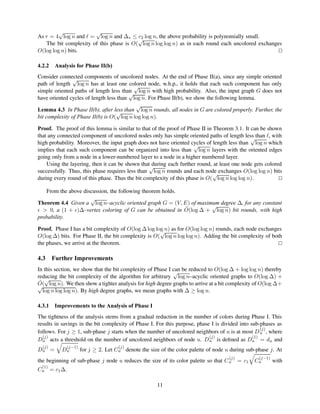
9. Colored node
Uncolored node
Legend:
11
2
1
2
3
3
3
3
Figure 3: Connected component of uncolored nodes. The number at the uncolored nodes within the con-
nected component gives the layer number they belong to.
Now, in Phase II, during every round the uncolored nodes assigned to the lowest layer number presently
get colored as the nodes assigned to the lowest layer can always retain their color choice from Step 1. This
implies that Phase II can finish in less than
√
log n rounds.
Since in each round each uncolored node has to exchange O(log ∆) = O(1) bits, the bit complexity of
the algorithm Color-Random is O(
√
log n).
We note that the same proof also holds for 3–coloring cycle graphs, with any orientation, with minimal
changes. Coupled with the lower bound result in Theorem 2.2, our analysis for the case of constant degree
graphs is tight with respect to the bit complexity, up to constant factors. The algorithm and the analysis can
be modified easily to achieve a local coloring also.
4 Upper Bound for Arbitrary Oriented Graphs
In this section we describe and analyze our algorithm for vertex coloring an arbitrary
√
log n–acyclic ori-
ented graph G using (1 + )∆ colors for any constant > 0.
Our algorithm and the analysis in this case requires more tools than that for constant degree graphs
while having the same flavor. Theorem 3.1 fails to hold once the degree of the input graph is bounded away
from any constant. Graphs below logarithmic degree, but bounded away from a constant, pose additional
problems as graphs with degree below a certain threshold are not easily amenable to nice probabilistic
bounds. In many papers, for example [12, 26, 5], this problem was overcome by assuming that the number
of colors available is max{(1 + )∆, log n} so that sub-logarithmic degree graphs are colored with log n
colors. We instead take the approach of coloring with (1 + )∆ colors as coloring with few colors is more
appealing when vertex coloring is used as a sub-routine in other higher order tasks.
To arrive at our result, we proceed in stages. Based on techniques from [12], we first show how to arrive
at a bit complexity of ˜O(log ∆ +
√
log n). Later, using advanced techniques, we show how to arrive at a bit
complexity of O(log ∆) + ˜O(
√
log n). Finally, for graphs with ∆ ≥ log n, we show how to arrive at a bit
complexity of O(log ∆ +
√
log n log log n).
Our algorithm for any node u is presented in Figure 4. The parameter Cu denotes the number of colors
each vertex u can choose from. Each node runs the algorithm in Figure 4 while it remains uncolored.
We now provide a summary of our analysis of algorithm Color. Our analysis cuts time into two phases.
In the first phase we show that for any vertex the number of uncolored neighbors reduces to at most c2 log n
for a constant c2, in O(log log n) rounds, with high probability. In the second phase we first show that the
graph can be decomposed into connected components of uncolored nodes such that each such connected
8

10. Algorithm Color(Cu)
Phase I
1. Set Cu := c1∆ for a constant c1 ≥ 3.
2. While du ≥ c2 log n for a constant c2 do
3. Use Algorithm Color-Random(Cu).
Phase II
4. Set Cu := min{2c2 log n, 2du}.
5. Use Algorithm Color-Random(Cu).
Figure 4: Algorithm for any node u.
component only has simple oriented paths of length less than
√
log n, with high probability. The analysis
then proceeds to show that all the nodes can be colored in a further
√
log n rounds.
In the algorithm and the analysis we also set Cu = c1∆ for a constant c1 ≥ 3, for every node u, for the
sake of simplicity. Using techniques from [12], it is possible to extend the following analysis to use only
(1 + )∆ colors, for any constant > 0.
4.1 Analysis for Phase I
In this phase, we show that the number of uncolored neighbors of any node u reduces in a double-exponential
fashion, (i.e., in O(log log n) rounds) to c2 log n. This analysis has strong connections to occupancy prob-
lems [25, Problem 3.4],[2], and the edge coloring algorithm of [12].
Let du(i), Nu(i), Cu(i) refer to the number of uncolored neighbors, the set of uncolored neighbors, and
the size of the color palette of node u respectively, at the beginning of round i. Also, let ˆd(i) = maxu du(i).
Lemma 4.1 If du(1) ≥ c2 log n then du(c log log n) ≤ c2 log n, with high probability for some constant
c ≥ 1.
Proof. The intuition behind the proof is that at the end of every round, the number of remaining uncolored
neighbors decreases double-exponentially.
During round i the probability that an uncolored node u fails to get colored can be computed as: Pu(i) :=
Pr[u does not get colored during round i] ≤
du(i)
j=1
1
Cu(i) ≤
ˆd(i)
α∆ , as, for c1 sufficiently large, it holds that
Cu(i) ≥ α∆ for α = c1 − 1.
The expected number of neighbors of u that are still uncolored after round i is, E[du(i + 1)] =
v∈Nu(i) Pv(i) ≤ ˆd(i)2/α∆.
Consider the following recurrence relation between ˆd(i + 1) and ˆd(i) for a constant c .
ˆd(i + 1) ≤
ˆd2(i)
α∆
+ c ˆd(i) log n. (1)
Using a large deviation bound [11, 12], it can be shown that du(i + 1) exceeds its expected value by
more than c ˆd(i) log n with probability less than n−2 for some constant c . Thus, it holds that du(i+1) ≤
ˆd(i + 1) w.h.p., for all nodes u.
The recurrence relation in Equation (1) can be solved as follows (cf. [12]). While ˆd2(i)/α∆ dominates
the second term, we can write:
ˆd(i + 1) ≤ 2 ˆd2
(i)/α∆ (2)
9

11. and find a value of r1 such that ˆd2(i)/α∆ ≤ 2 c ˆd(i) log n. For this we require that ˆd3(r1) ≤ 4c α2∆2 log n.
Using Equation (2), it follows that
ˆd(r1) ≤ (2/α)2r1−1
∆
Hence, we require that:
(2/α)2r1−1
∆
3
= 4α2
∆2
c log n
which results in a value of r1 = O(log log n).
From this point on, it holds that
ˆd(i + 1) ≤ 8 c ˆd(i) log n (3)
Solving Equation (3) for a value of r2 so that ˆd(r2) ≤ c2 log n results in r2 = O(log log n).
Thus after i∗ = r1 + r2 = O(log log n) rounds, we have for any node u, du(i∗) ≤ ˆd(i∗) ≤ c2 log n.
Thus, at the end of O(log log n) rounds of the algorithm, the number of uncolored neighbors for every
node is at most c2 log n. This completes Phase I of the analysis.
4.2 Analysis for Phase II
The analysis in this phase consists of two sub-phases. In sub-phase II(a), we argue that along any simple
oriented path of length
√
log n there exists at least one colored node, with high probability. In the second
sub-phase we show that all the remaining uncolored nodes successfully get colored within
√
log n rounds.
Notice that since the number of uncolored neighbors of any node at the beginning of this phase is at most
c2 log n, nodes can use a color palette of size min{2c2 log n, 2du} for this phase as shown in the algorithm
in Figure 4.
4.2.1 Analysis for Phase II(a)
We now establish the following lemma which shows that every simple oriented path of length
√
log n has at
least one colored node after O(
√
log n) rounds, with high probability. Let ∆∗ denote the maximum number
of uncolored neighbors for any node u. After phase I, it holds that ∆∗ ≤ c2 log n.
Lemma 4.2 For arbitrary
√
log n–acyclic oriented graphs G at the end of O(
√
log n) rounds, any simple
oriented path of length =
√
log n will have at least one colored node, with high probability. Further, the
bit complexity of this phase is O(
√
log n log log n).
Proof. The proof of this lemma is similar to the proof of Phase I of Theorem 3.1. Consider any simple
oriented path P of length =
√
log n. Let EP,i denote the event that all the nodes in P are in a color conflict
during a given round i. Then, along the lines of Phase I of Theorem 3.1, it holds that Pr[EP,i | ∩i−1
j=1EP,j] ≤
(1/2) . Define EP to be the event that the event EP,i occurs for r = 4
√
log n consecutive rounds. Then, it
holds that
Pr[EP ] = Pr[∩r
i=1EP,i] = Πr
i=1 Pr[EP,i | ∩i−1
j=1EP,j] ≤ (1/2) r
.
Let E denote the event that there exists a path P for which the event EP occurs. Since the number of
simple oriented paths of length P is at most n∆∗,
Pr[E] ≤
P
Pr[EP ] ≤ n∆∗
1
2
r
.
10

12. As r = 4
√
log n and =
√
log n and ∆∗ ≤ c2 log n, the above probability is polynomially small.
The bit complexity of this phase is O(
√
log n log log n) as in each round each uncolored exchanges
O(log log n) bits.
4.2.2 Analysis for Phase II(b)
Consider connected components of uncolored nodes. At the end of Phase II(a), since any simple oriented
path of length
√
log n has at least one colored node, w.h.p., it holds that each such component has only
simple oriented paths of length less than
√
log n with high probability. Also, the input graph G does not
have oriented cycles of length less than
√
log n. For Phase II(b), we show the following lemma.
Lemma 4.3 In Phase II(b), after less than
√
log n rounds, all nodes in G are colored properly. Further, the
bit complexity of Phase II(b) is O(
√
log n log log n).
Proof. The proof of this lemma is similar to that of the proof of Phase II in Theorem 3.1. It can be shown
that any connected component of uncolored nodes only has simple oriented paths of length less than , with
high probability. Moreover, the input graph does not have oriented cycles of length less than
√
log n which
implies that each such component can be organized into less than
√
log n layers with the oriented edges
going only from a node in a lower-numbered layer to a node in a higher numbered layer.
Using the layering, then it can be shown that during each further round, at least one node gets colored
successfully. Thus, this phase requires less than
√
log n rounds and each node exchanges O(log log n) bits
during every round of this phase. Thus the bit complexity of this phase is O(
√
log n log log n).
From the above discussion, the following theorem holds.
Theorem 4.4 Given a
√
log n–acyclic oriented graph G = (V, E) of maximum degree ∆, for any constant
> 0, a (1 + )∆–vertex coloring of G can be obtained in ˜O(log ∆ +
√
log n) bit rounds, with high
probability.
Proof. Phase I has a bit complexity of O(log ∆ log log n) as for O(log log n) rounds, each node exchanges
O(log ∆) bits. For Phase II, the bit complexity is O(
√
log n log log n). Adding the bit complexity of both
the phases, we arrive at the theorem.
4.3 Further Improvements
In this section, we show that the bit complexity of Phase I can be reduced to O(log ∆ + log log n) thereby
reducing the bit complexity of the algorithm for arbitrary
√
log n–acyclic oriented graphs to O(log ∆) +
˜O(
√
log n). We then show a tighter analysis for high degree graphs to arrive at a bit complexity of O(log ∆+√
log n log log n). By high degree graphs, we mean graphs with ∆ ≥ log n.
4.3.1 Improvements to the Analysis of Phase I
The tightness of the analysis stems from a gradual reduction in the number of colors during Phase I. This
results in savings in the bit complexity of Phase I. For this purpose, phase I is divided into sub-phases as
follows. For j ≥ 1, sub-phase j starts when the number of uncolored neighbors of u is at most D
(j)
u , where
D
(j)
u acts a threshold on the number of uncolored neighbors of node u. D
(j)
u is defined as D
(1)
u = du and
D
(j)
u = D
(j−1)
u for j ≥ 2. Let C
(j)
u denote the size of the color palette of node u during sub-phase j. At
the beginning of sub-phase j node u reduces the size of its color palette so that C
(j)
u = c1 C
(j−1)
u with
C
(1)
u = c1∆.
11

13. Algorithm PhaseI
1. Du :=
√
du, Cu := c1∆.
2. While du ≥ c2 log n do
3. Run Algorithm Color–Random(Cu).
4. If du ≤ Du then
5. Du :=
√
Du, Cu := c1
√
Cu
end-while.
Figure 5: Improved algorithm for Phase I.
This effectively reduces the number of bits required to be sent in each sub-phase by a factor of 2 but the
proof of Lemma 4.1 holds with minimal changes. Thus, in Phase I, it can be seen that over the O(log log n)
sub-phases the number of bits each node u sends is at most
O(log log n)
j=1
log C(j)
u ≤
O(log log n)
j=1
2 log c1 + ((log ∆)/2j
) = O(log log n + log ∆).
Thus, the bit complexity for Phase I reduces to O(log log n + log ∆).
The modified algorithm for Phase I for node u is described in Figure 5. Using the tighter analysis for
Phase I and Lemmata 4.2–4.3, we arrive at the following theorem.
Theorem 4.5 Given a
√
log n–acyclic oriented graph G = (V, E) of maximum degree ∆, a (1 + )∆–
vertex coloring of G for any constant > 0, can be obtained in O(log ∆) + ˜O(
√
log n) bit rounds, with
high probability.
4.3.2 Improvements to Phase II
For the case of high degree graphs, we now show how to reduce the bit complexity of Phase II to O(
√
log n log log n).
The algorithm for Phase II remains the same as shown in Figure 4. The analysis of Phase II now consists
of 3 sub-phases. In sub-phase II(a), we show that the number of uncolored neighbors of any node decreases
to O(
√
log n log log n) after O(
√
log n/ log log n) rounds with high probability. In sub-phase II(b) we then
show that every simple oriented path of length log n/ log log n has at least one colored node, with high
probability, after O( log n/ log log n) rounds. In the final sub-phase, we show that every node can be
colored in a further O( log n/ log log n) rounds. In this phase, every node can use a color palette of size
2c2 log n.
Analysis for Phase II(a)
For sub-phase II(a), we show the following lemma.
Lemma 4.6 In Phase II(a), in O(
√
log n
log log n ) rounds, the number of uncolored neighbors of any node decreases
to
√
log n log log n, with high probability. Further, the bit complexity of this sub-phase is O(
√
log n).
Proof. Consider any node u. At the end of phase I, it holds that du ≤ c2 log n, with high probability. Since
the number of colors used by u is 2c2 log n, it also holds that
Pr[node u fails to get colored in a given round] ≤ 1/2.
12

14. Consider any subset A of the uncolored neighbors of u. Let EA denote the event that all the nodes in A
remain uncolored after r = 4
√
log n
log log n consecutive rounds. Then, it holds that
Pr[EA] ≤ (1/2)r|A|(1−1/
√
log n)
using the orientation and the witnessing scheme of Theorem 3.1. Notice that as we are guaranteed of√
log n–acyclicity we can find a set of at least |A|(1 − 1/
√
log n) nodes in conflict with a distinct witness
for each color conflict.
Let Eu,s denote the event that for node u, there exists a set of s uncolored neighbors at the end of r
rounds. Then,
Pr[Eu,s] = Pr[
A⊆Nu,|A|=s
EA] ≤
A⊆Nu,|A|=s
Pr[EA] =
du
s
1
2
rs(1−1/
√
log n)
.
Denote by Eu the event that for node u there exist more than
√
log n log log n uncolored neighbors.
Using Boole’s inequality,
Pr[Eu] ≤
du
s=
√
log n log log n
Pr[Eu,s] ≤
du
s=
√
log n log log n
du
s
·(1/2)rs(1−1/
√
log n)
≤ 2du
·(1/2)3 log n
≤
1
n2
.
as rs ≥ 4 log n. Now, denote by E the event that for some node u, the event Eu occurs. Then, Pr[E] =
Pr[ u∈V Eu] ≤ 1/n. Thus, the number of uncolored neighbors of any node decreases to
√
log n log log n
with high probability after 4
√
log n/ log log n rounds.
During this phase, each uncolored node exchanges O(log log n) bits in each round as the palette size is
2c2 log n. Thus, the bit complexity of this sub-phase is O(
√
log n).
Analysis for Phase II(b)
At the end of sub-phase II(a), it holds that the number of uncolored neighbors of any node u is at most√
log n log log n. Recall that ∆∗ = maxu du. After sub-phase II(a), it holds that ∆∗ ≤
√
log n log log n.
Lemma 4.7 In Phase II(b), in 16 log n/ log log n rounds, in every simple oriented path of length log n/ log log n
there is at least one node that gets colored, with high probability. Further, the bit complexity of this sub-
phase is O(
√
log n log log n).
Proof. Consider any simple oriented path P of uncolored nodes of length = log n/ log log n. Denote
by EP the event that no node in P gets colored in 16 log n/ log log n rounds. Since P is oriented and the
choices of each node are independent, using a witnessing scheme similar to that in the proof of Theorem
3.1, it holds that:
Pr[EP ] ≤
√
log n log log n
2c2 log n
·16
√
log n/ log log n
≤
log log n
2c2
√
log n
16 log n
log log n
≤
1
n4
,
if n is sufficiently large. In the above, the first inequality holds since the number of uncolored neighbors is√
log n log log n and the number of colors that u can choose from is 2c2 log n.
Let E denote the event that there exists a simple oriented path P of length such that for path P, the
event EP occurs. The number of simple oriented paths of length = log n/ log log n is at most n · ∆∗.
Thus,
13

15. Pr[E] = Pr[
P
EP ] ≤
n∆∗
j=1
1/n4
≤ ∆∗/n3
.
The above probability is polynomially small since ∆∗ ≤
√
log n log log n. Thus, along any simple
oriented path of length log n/ log log n, at least one node gets colored with high probability at the end of
16 log n/ log log n rounds.
The bit complexity of this sub-phase is easily seen to be O(
√
log n log log n) as in each round, each
uncolored node exchanges O(log log n) bits.
This completes the analysis for Phase II(b). In Phase II(c), using arguments similar to that of Lemma 4.3,
it can be shown that in a further log n/ log log n rounds, every node gets colored, with high probability.
The bit complexity of Phase II(c) is O(
√
log n log log n). Putting together everything, we arrive at the
following theorem.
Theorem 4.8 Given a
√
log n–acyclic oriented graph G = (V, E) of maximum degree ∆ ≥ log n, for any
constant > 0, a (1+ )∆–vertex coloring of G can be obtained in O(log ∆+
√
log n log log n) bit rounds,
with high probability.
Notice that for Theorem 4.8 to hold, the input graph only needs to be log n/ log log n–acyclic, but we
stated the theorem with the
√
log n–acyclicity assumption for the sake of consistency.
The following corollary can be easily obtained showing that for the case of dense
√
log n–acyclic ori-
ented graphs, our result on the bit complexity is close to the worst-case optimal.
Corollary 4.9 Given an arbitrary
√
log n–acyclic oriented graph G = (V, E) with ∆ = Ω(2
√
log n log log n),
for any > 0, a (1 + )∆-vertex coloring can be obtained in O(log ∆) bit rounds, with high probability.
5 Conclusions
We presented algorithms for distributed vertex coloring using a simple and natural model. While our results
are tight in general, a related question to ask is whether any further conditions on the orientation would
result in better bounds or whether certain orientations outperform other orientations. For example, if the
orientation or the graph is known to be acyclic, would it be possible to color in fewer bit rounds?
References
[1] L. Barriere, P. Flocchini, P. Fraigniaud, and N. Santoro. Can we elect if we cannot compare? In Proc.
of the ACM Symposium on Parallelism in Algorithms and Architectures (SPAA), pages 324–332, 2003.
[2] M. Bender, M. Farach-Colton, S. He, B. Kuszmaul, and C. Leiserson. Adversarial contention resolu-
tion for simple channels. In Proc. of ACM Symposium on Parallelism in Algorithms and Architectures
(SPAA), pages 325–332, 2005.
[3] M. Choy and A. K. Singh. Efficient fault tolerant algorithms for resource allocation in distributed
systems. In Proc. of the ACM Symposium on Theory of Computing (STOC), pages 169–177, 1992.
[4] R. Cole and U. Vishkin. Deterministic coin tossing and accelerating cascades: micro and macro
techniques for designing parallel algorithms. In Proc. of the ACM Symposium on Theory of Computing
(STOC), pages 206–219, 1986.
14

16. [5] D. P. Dubhashi and A. Panconesi. Near-optimal distributed edge coloring. In Proc. of the European
Symposium on Algorithms (ESA), pages 448–459, 1995.
[6] U. Feige and J. Kilian. Zero-knowledge and chromatic number. In Proc. of the Annual Conference on
Computational Complexity, 1996.
[7] I. Finocchi, A. Panconesi, and R. Silvestri. Experimental analysis of simple, distributed vertex coloring
algorithms. In Proc. of the ACM Symposium on Discrete Algorithms (SODA), pages 606–615, 2002.
[8] P. Flocchini, B. Mans, and N. Santoro. On the impact of sense of direction on message complexity.
Information Processing Letters, 63(1):23–31, 1997.
[9] M. R. Garey and D. S. Johnson. Computers and Intractability: A guide to the theory of NP-
completeness. W.H. Freeman, 1979.
[10] A. Goldberg, S. Plotkin, and G. Shannon. Parallel symmetry breaking in sparse graphs. SIAM J.
Discrete Math., 1:434–446, 1989.
[11] D. A. Grable. A large deviation inequality for functions of independent, multi-way choices. Comb.
Probab. Comput., 7(1), 1998.
[12] D. A. Grable and A. Panconesi. Nearly optimal distributed edge colouring in O(log log n) rounds.
Random Structures and Algorithms, 10(3):385–405, 1997.
[13] C. Intanagonwiwat, R. Govindan, and D. Estrin. Directed diffusion: A scalable and robust commu-
nication paradigm for sensor networks. In Proc. of the 6th ACM/IEEE Mobicom Conference, pages
56–67, 2000.
[14] O. Johansson. Simpled distributed ∆ + 1 coloring of graphs. Information Processing Letters, 70:229–
232, 1999.
[15] M. Karchmer and J. Naor. A fast parallel algorithm to color a graph with ∆ colors. J. Algorithms,
9:83–91, 1988.
[16] R. Karp and A. Widgerson. A fast parallel algorithm for the maximal independent set problem. Journal
of the Association for Computing Machinery, 32(4):762–773, 1985.
[17] K. Kothapalli, M. Onus, A. Richa, and C. Scheideler. Constant density spanners for wireless ad-hoc
networks. In Proc. of the ACM Symposium on Parallelism in Algorithms and Architectures (SPAA),
pages 116–125, 2005.
[18] K. Kothapalli, M. Onus, C. Scheideler, and C. Schindelhauer. Distributed coloring in ˜O(
√
log n)–bits.
In Proc. of IEEE International Parallel and Distributed Processing Symposium (IPDPS), 2006.
[19] K. Kothapalli and C. Scheideler. Information gathering in adversarial systems: Lines and cycles. In
Proc. of the ACM Symposium on Parallelism in Algorithms and Architectures (SPAA), pages 333–342,
2003.
[20] V. Kumar, M. Marathe, S. Parthasarathy, and A. Srinivasan. End-to-end packet-scheduling in wireless
ad-hoc networks. In Proc. of ACM Symposium on Discrete Algorithms (SODA), pages 1021–1030,
2004.
[21] N. Linial. Locality in distributed graph algorithms. SIAM Journal of Computing, 21:193–201, 1992.
15

17. [22] M. Luby. A simple parallel algorithm for the maximal independent set problem. In Proc. of the 17th
ACM Symposium on Theory of Computing (STOC), pages 1–10, 1985.
[23] M. Luby. Removing randomness in parallel without processor penalty. Journal of Computer and
System Sciences, 47(2):250–286, 1993.
[24] G. De Marco and A. Pelc. Fast distributed graph coloring with O(∆) colors. In Proc. of ACM Sympo-
sium on Discrete Algorithms (SODA), pages 630–635, 2001.
[25] R. Motwani and P. Raghavan. Randomized Algorithms. Cambridge University Press, 1995.
[26] A. Panconesi and A. Srinivasan. Fast randomized algorithms for distributed edge coloring. In Proc. of
the ACM Symposium on Principles of Distributed Computing (PODC), pages 251–262, 1992.
[27] A. Panconesi and A. Srinivasan. On the complexity of distributed network decomposition. J. Algo-
rithms, 20(2):356–374, 1996.
[28] G. Singh. Efficient leader election using sense of direction. Distributed Computing, 10(3):159–165,
1997.
16