Lecture 5b graphs and hashing

GRAPHS - INTRODUCTION
 Many real-life problems can be formulated in terms
of sets of objects and relationships or connections
between objects. Examples include:
 Finding routes between cities: the objects could be
towns, and the connections could be road/rail links.
 Deciding what first year courses to take: the
objects are courses, and the relationships are
prerequisite and co requisite relations. Similarly,
planning a course: the objects are topics, and the
relations are prerequisites between topics (you
have to understand topic X before topic Y will
make sense).

DEFINITIONS
 A graph is a data structure (ADT) that consists
of a set of vertices (or nodes) (which can
represent objects), and a set of edges linking
vertices (which can represent relationships
between the objects).
 A tree is a special kind of graph (with certain
restrictions).
 Graph algorithms operate on a graph data
structure, and allow us to, for example, search
a graph for a path between two given nodes;
find the shortest path between two nodes; or
order the vertices in the graph is a particular
way.

DEFINITIONS……
 A graph is a generalization of the tree
structure, where instead of a strict parent/child
relationship between tree nodes, any kind of
complex relationships between the nodes can
be represented.
 The graph ADT follows directly from the
GRAPH concept from mathematics.

DEFINITIONS.....
 Incident edge: (vi,vj) is an edge, then edge(vi,vj)
is said to be incident to vertices vi and vj
 If vi and vj are connected, they are said to be
adjacent vertices/nodes
 vi and vj are endpoints of the edge {vi, vj}
 If an edge e is connected to v, then v is said to
be incident on e. Also, the edge e is said to be
incident on v.

DEFINITIONS
 Cycle
 Path that ends back at the starting node
 Example:
A, B, C, G, AA, B, C, G, A
 Simple path
 No cycles in path
 Acyclic graph
 Graph with no cycles
 Acyclic undirected graphs are trees
GG
CCBB
AA
HH NN
KK

UnconnectedUnconnected
graph withgraph with
two connectedtwo connected
componentscomponents
DEFINITIONS
 Two nodes are reachable if
 Path exists between them
 Connected graph
 Every node is reachable from any other node
GG
JJ
FF
DD
AA
Connected graphConnected graph
GG
JJ
FF
DD
AA
EE
CC HH

Degree of vertex.....
 The number of edges incident onto the vertex
For a directed graph:
 In degree of a vertex vi is the number of
edges incident onto vi, with vi as the head.
 Out degree of vertex vi is the number of
edges incident onto vi, with vi as the tail.
 In a directed graph, the number of edges that
point to a given vertex is called its in-degree,
and the number that point from it is called its
out-degree.

Directed/Digraph Graph
 Origin and terminating nodes
 A graph is connected if there is a path between
any two vertices.
 A directed graph is strongly connected if there
is a directed path between any two vertices
(edges have directions).
 The degree of a vertex is the number of edges
adjacent to it.

Undirected (Undigraph)Graph
 A graph is undirected if (x,y) implies (y,x).
 An edge of the form (x,x) is said to be a
loop.
 If x is y's friend several times over, that
could be modeled using multiedges,
multiple edges between the same pair of
vertices.
 A graph is said to be simple if it contains
no loops and multiple edges.

…….
 A path is a sequence of edges connecting
two vertices.
 Since Brooks is my father's-sister's-
husband's cousin, there is a path between
me and him! Etc.

Graphs
 Directed graph
 Edges have
direction
 Undirected graphUndirected graph
 Undirected edgesUndirected edges
77
1919
2121
11
1212
44
33
2222
22
33
GG
JJ
FF
DD
AA
EE CC HH
12

Weighted graph
 Weight (cost) is associated with each
edge
GG
JJ
FF
DD
AA
EE CC HH
QQ
KK
NN
10
4
14
6 16
9
8
7
5
22
3
13

Edges are of 2 types
 Directed edge: A directed edge between the
vertices vi and vj is an ordered pair. It is
denoted by <vi,vj>.
 Undirected edge: An undirected edge between
the vertices vi and vj is an unordered pair. It is
denoted by (vi,vj).
 Maximum number of edges: The maximum
number of edges in an undirected graph with n
vertices is n(n−1)/2.
 In a directed graph, it is n(n−1).

PATHS
 Path (in directed graph)
 Examples:
A, B, C is a path
A, G, K is not a path
GG
CCBB
AA
HH NN
KK

PATHS
 Path in undirected graph
 Examples:
A, B, C is a path
H, K, C is not a path
GG
CCBB
AA
HH NN
KK
16

Representing Graphs
 Adjacency list
 Each node holds a
list of its neighbors
 Adjacency matrix
 Each cell keeps
whether and how two
nodes are connected
 Set of edges
00 11 00 11
00 00 11 00
11 00 00 00
00 11 00 00
1
2
3
4
1 2 3 4
{1,2} {1,4} {2,3} {3,1} {4,2}{1,2} {1,4} {2,3} {3,1} {4,2}
11  {2,{2,
4}4}
22  {3}{3}
33  {1}{1}
44  {2}{2}
22
4411
33
17

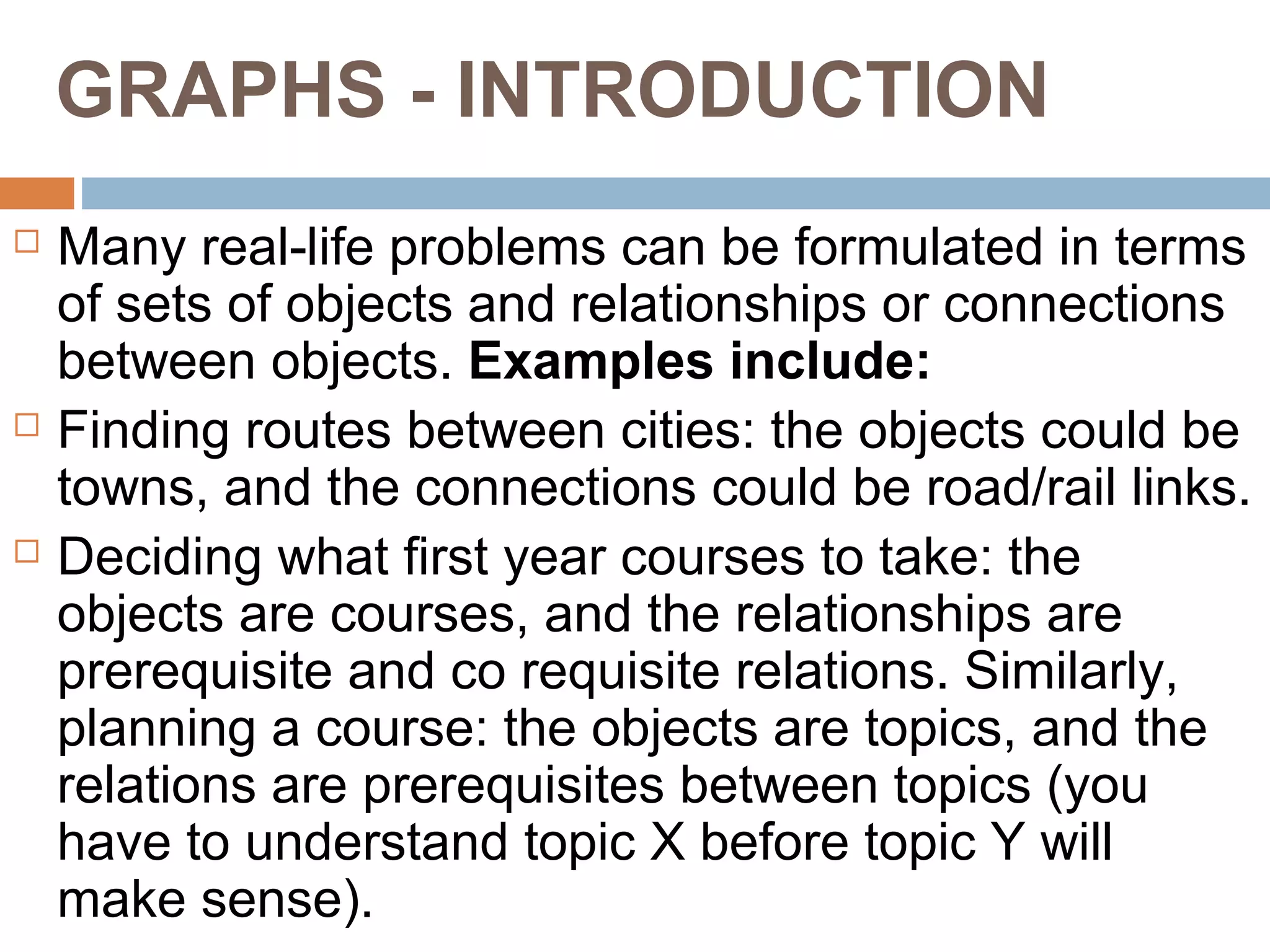
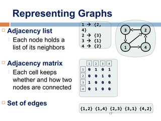
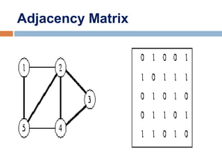
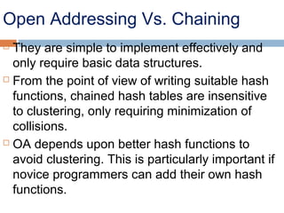
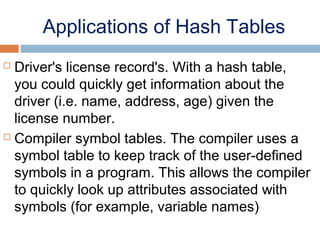
Adjacency Matrix
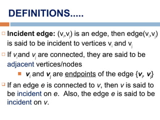
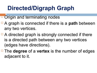
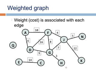
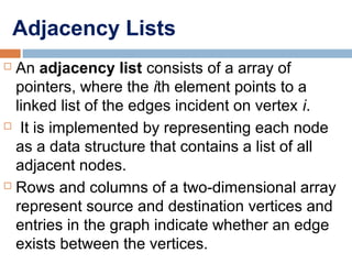
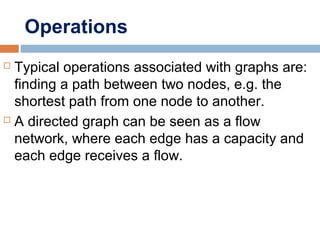
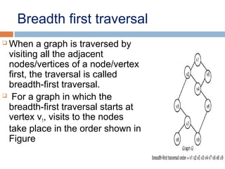
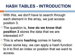
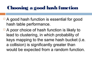
• 2D array, where n is the number of vertices in the graph
• Each row and column is indexed by the vertex id.
- e,g a=0, b=1, c=2, d=3, e=4
• An array entry A [i] [j] is equal to 1 if there is an edge
connecting
vertices i and j. Otherwise, A [i] [j] is 0.

Adjacency Matrix
2
4
3
5
1
7
6
9
8
0
0 1 2 3 4 5 6 7 8 9
0 0 0 0 0 0 0 0 0 1 0
1 0 0 1 1 0 0 0 1 0 1
2 0 1 0 0 1 0 0 0 1 0
3 0 1 0 0 1 1 0 0 0 0
4 0 0 1 1 0 0 0 0 0 0
5 0 0 0 1 0 0 1 0 0 0
6 0 0 0 0 0 1 0 1 0 0
7 0 1 0 0 0 0 1 0 0 0
8 1 0 1 0 0 0 0 0 0 1
9 0 1 0 0 0 0 0 0 1 0

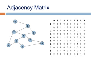
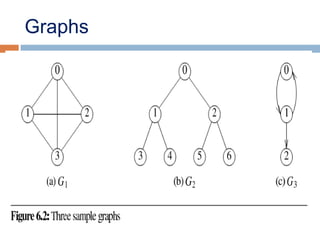
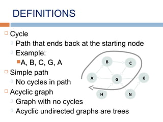
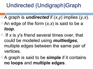
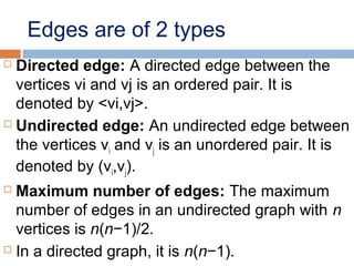
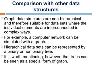
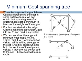
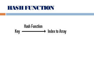
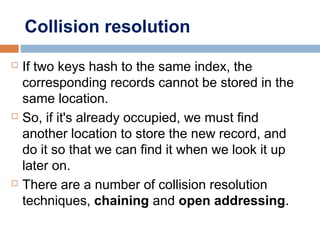
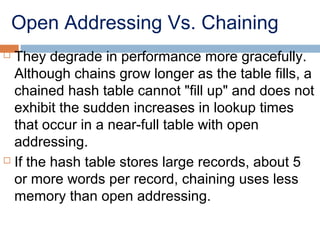
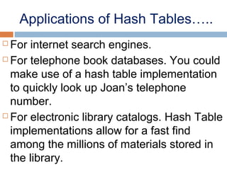
Adjacency List
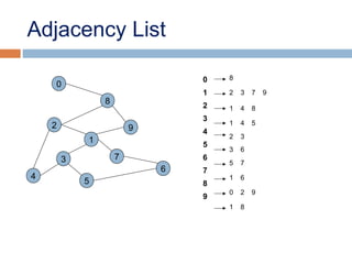
• The adjacency list is an array A[0..n-1] of lists, where n is the
number of vertices in the graph.
•Each array entry is indexed by the vertex id (as with adjacency
matrix)
• The list A[i] stores the ids of the vertices adjacent to i.

Adjacency Lists
 An adjacency list consists of a array of
pointers, where the ith element points to a
linked list of the edges incident on vertex i.
 It is implemented by representing each node
as a data structure that contains a list of all
adjacent nodes.
 Rows and columns of a two-dimensional array
represent source and destination vertices and
entries in the graph indicate whether an edge
exists between the vertices.

Adjacency List
2
4
3
5
1
7
6
9
8
0
0
1
2
3
4
5
6
7
8
9
2 3 7 9
8
1 4 8
1 4 5
2 3
3 6
5 7
1 6
0 2 9
1 8

Adjacency Multi list
 In the adjacency-list representation, each edge
(u, v) is represented by two entries, one on the
list for u and the other on the list for v
 Multi lists: lists in which nodes may be shared
among several lists
 For each edge there will be exactly one node,
but this node will be in two lists (i.e., the
adjacency lists for each of the two nodes to
which it is incident)

Adjacency Lists vs. Matrix
 Adjacency Lists
 More compact than adjacency matrices if
graph has few edges
 Requires more time to find if an edge
exists
 Adjacency Matrix
 Always require n2
space
This can waste a lot of space if the
number of edges are sparse
 Can quickly find if an edge exists

Operations
 Typical operations associated with graphs are:
finding a path between two nodes, e.g. the
shortest path from one node to another.
 A directed graph can be seen as a flow
network, where each edge has a capacity and
each edge receives a flow.

Comparison with other data
structures
 Graph data structures are non-hierarchical
and therefore suitable for data sets where the
individual elements are interconnected in
complex ways.
 For example, a computer network can be
simulated with a graph.
 Hierarchical data sets can be represented by
a binary or non binary tree.
 It is worth mentioning, however, that trees can
be seen as a special form of graph.

Graph traversal
Traversal of graph implies visiting the nodes
of the graph.
A graph can be traversed in 2 ways
 Depth first traversal
 Breadth first traversal

Depth First traversal
 When a graph is traversed by
visiting the nodes in the
forward (deeper) direction as
long as possible, the traversal
is called depth-first traversal.
 E.g. the depth-first traversal
starting at the vertex 0 visits
the node in the orders:
 0 1 2 6 7 8 5 3 4
 0 4 3 5 8 6 7 2 1

Breadth first traversal
 When a graph is traversed by
visiting all the adjacent
nodes/vertices of a node/vertex
first, the traversal is called
breadth-first traversal.
 For a graph in which the
breadth-first traversal starts at
vertex v1, visits to the nodes
take place in the order shown in
Figure

Minimum Cost spanning tree
 When the edges of the graph have
weights representing the cost in
some suitable terms, we can
obtain that spanning tree of a
graph whose cost is minimum in
terms of the weights of the edges.
 For this, we start with the edge
with the minimum-cost/weight, add
it to set T, and mark it as visited.
 We next consider the edge with
minimum-cost that is not yet
visited, add it to T, and mark it as
visited. While adding an edge to
the set T, we first check whether
both the vertices of the edge are
visited; if they are, we do not add
to the set T, because it will form a
cycle.
The minimum-cost spanning tree of the graph
is as shown

BFS and Shortest Path Problem
 Given any source vertex s, BFS visits the other vertices at
increasing distances away from s. In doing so, BFS discovers
paths from s to other vertices
 What do we mean by “distance”? The number of edges on a
path from s.
2
4
3
5
1
7
6
9
8
0
Consider s=vertex 1
Nodes at distance 1?
2, 3, 7, 91
1
1
1
2
22
2
s
Example
8, 6, 5, 4
0

Graphs and Their Applications
 Graphs have many real-world applications
 Modeling a computer network like Internet
Routes are simple paths in the network
 Modeling a city map
Streets are edges, crossings are vertices
 Social networks
People are nodes and their connections are
edges
 State machines
States are nodes, transitions are edges

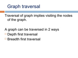
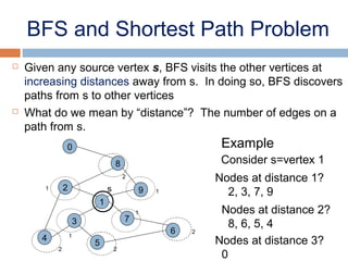
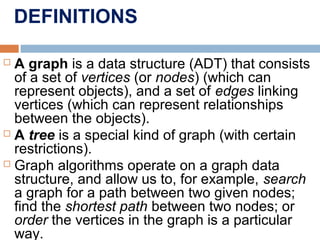
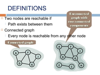
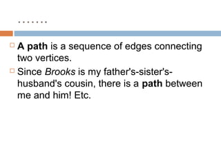
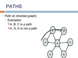
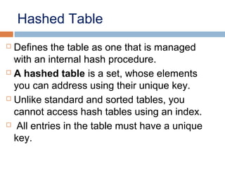
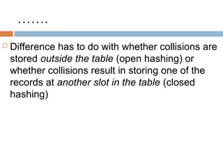
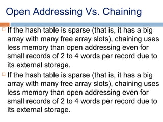
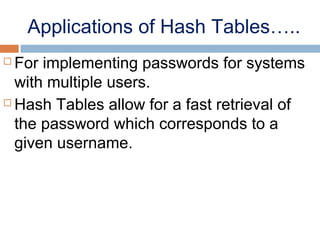
Representing Graphs in C#
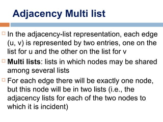
public class Graphpublic class Graph
{{
int[][] childNodes;int[][] childNodes;
public Graph(int[][] nodes)public Graph(int[][] nodes)
{{
this.childNodes = nodes;this.childNodes = nodes;
}}
}}
Graph g = new Graph(new int[][] {Graph g = new Graph(new int[][] {
new int[] {3, 6}, // successors of vertice 0new int[] {3, 6}, // successors of vertice 0
new int[] {2, 3, 4, 5, 6}, // successors of vertice 1new int[] {2, 3, 4, 5, 6}, // successors of vertice 1
new int[] {1, 4, 5}, // successors of vertice 2new int[] {1, 4, 5}, // successors of vertice 2
new int[] {0, 1, 4} // successors of vertice 6new int[] {0, 1, 4} // successors of vertice 6
});});
00
66
44
11
55
22
33

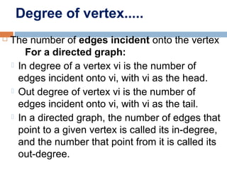
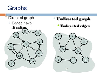
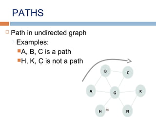
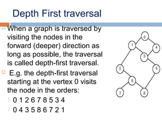
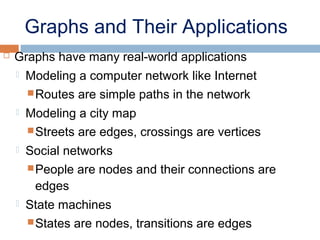
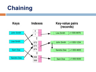
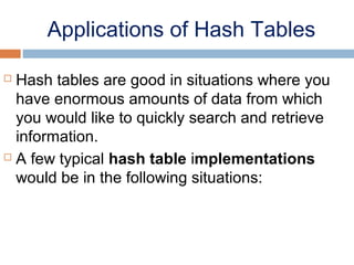
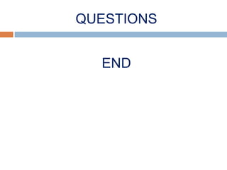
HASH TABLES - INTRODUCTION
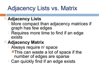
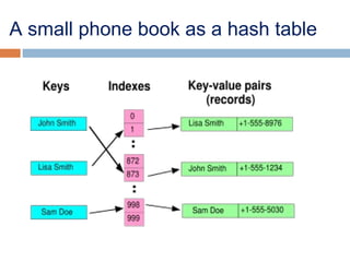
 WHY the use of Hash tables
 Hash tables are good for doing a quick
search on things.
 For instance if we have an array full of data
(say 100 items). If we knew the position that a
specific item is stored in an array, then we
could quickly access it.
 For instance, we just happen to know that the
item we want is at position 3; I can apply:
myitem=myarray[3];

HASH TABLES - INTRODUCTION
 With this, we don't have to search through
each element in the array, we just access
position 3.
 The question is, how do we know that
position 3 stores the data that we are
interested in?
 This is where hashing comes in handy.
 Given some key, we can apply a hash function
to it to find an index or position that we want to
access.

Hashed Table
 Defines the table as one that is managed
with an internal hash procedure.
 A hashed table is a set, whose elements
you can address using their unique key.
 Unlike standard and sorted tables, you
cannot access hash tables using an index.
 All entries in the table must have a unique
key.

A small phone book as a hash table

Choosing a good hash function
 A good hash function is essential for good
hash table performance.
 A poor choice of hash function is likely to
lead to clustering, in which probability of
keys mapping to the same hash bucket (i.e.
a collision) is significantly greater than
would be expected from a random function.

Collision resolution
 If two keys hash to the same index, the
corresponding records cannot be stored in the
same location.
 So, if it's already occupied, we must find
another location to store the new record, and
do it so that we can find it when we look it up
later on.
 There are a number of collision resolution
techniques, chaining and open addressing.

…….
 Difference has to do with whether collisions are
stored outside the table (open hashing) or
whether collisions result in storing one of the
records at another slot in the table (closed
hashing)

Hash collision resolved by chaining
 In the simplest chained hash table technique,
each slot in the array references a linked list of
inserted records that collide to the same slot.
 Insertion requires finding the correct slot, and
appending to either end of the list in that slot;
deletion requires searching the list and
removal.
 Chained hash tables inherit the disadvantages
of linked lists.
 When storing small records, the overhead of
the linked list can be significant. Also,
traversing a linked list has poor cache

Open Addressing
 Open addressing hash tables can store
the records directly within the array.
 A hash collision is resolved by probing, or
searching through alternate locations in
the array (the probe sequence) until either
the target record is found, or an unused
array slot is found, which indicates that
there is no such key in the table.

Probe sequences include:
 Linear probing the interval between
probes is fixed--often at 1,
 Quadratic probing the interval between
probes increases linearly (hence, the
indices are described by a quadratic
function), and
 Double probing the interval between
probes is fixed for each record but is
computed by another hash function.

Open Addressing Vs. Chaining
 They are simple to implement effectively and
only require basic data structures.
 From the point of view of writing suitable hash
functions, chained hash tables are insensitive
to clustering, only requiring minimization of
collisions.
 OA depends upon better hash functions to
avoid clustering. This is particularly important if
novice programmers can add their own hash
functions.

 They degrade in performance more gracefully.
Although chains grow longer as the table fills, a
chained hash table cannot "fill up" and does not
exhibit the sudden increases in lookup times
that occur in a near-full table with open
addressing.
 If the hash table stores large records, about 5
or more words per record, chaining uses less
memory than open addressing.

 If the hash table is sparse (that is, it has a big
array with many free array slots), chaining uses
less memory than open addressing even for
small records of 2 to 4 words per record due to
its external storage.
 If the hash table is sparse (that is, it has a big
array with many free array slots), chaining uses
less memory than open addressing even for
small records of 2 to 4 words per record due to
its external storage.

Applications of Hash Tables
 Hash tables are good in situations where you
have enormous amounts of data from which
you would like to quickly search and retrieve
information.
 A few typical hash table implementations
would be in the following situations:

Applications of Hash Tables
 Driver's license record's. With a hash table,
you could quickly get information about the
driver (i.e. name, address, age) given the
license number.
 Compiler symbol tables. The compiler uses a
symbol table to keep track of the user-defined
symbols in a program. This allows the compiler
to quickly look up attributes associated with
symbols (for example, variable names)

Applications of Hash Tables…..
 For internet search engines.
 For telephone book databases. You could
make use of a hash table implementation
to quickly look up Joan’s telephone
number.
 For electronic library catalogs. Hash Table
implementations allow for a fast find
among the millions of materials stored in
the library.

Applications of Hash Tables…..
 For implementing passwords for systems
with multiple users.
 Hash Tables allow for a fast retrieval of
the password which corresponds to a
given username.

Lecture 5b graphs and hashing

More Related Content

What's hot

Similar to Lecture 5b graphs and hashing

More from Victor Palmar

Recently uploaded

Lecture 5b graphs and hashing