This paper discusses a GPU implementation of the Louvain community detection algorithm. Louvain algorithm obtains hierachical communities as a dendrogram through modularity optimization. Given an undirected weighted graph, all vertices are first considered to be their own communities. In the first phase, each vertex greedily decides to move to the community of one of its neighbours which gives greatest increase in modularity. If moving to no neighbour's community leads to an increase in modularity, the vertex chooses to stay with its own community. This is done sequentially for all the vertices. If the total change in modularity is more than a certain threshold, this phase is repeated. Once this local moving phase is complete, all vertices have formed their first hierarchy of communities. The next phase is called the aggregation phase, where all the vertices belonging to a community are collapsed into a single super-vertex, such that edges between communities are represented as edges between respective super-vertices (edge weights are combined), and edges within each community are represented as self-loops in respective super-vertices (again, edge weights are combined). Together, the local moving and the aggregation phases constitute a stage. This super-vertex graph is then used as input fof the next stage. This process continues until the increase in modularity is below a certain threshold. As a result from each stage, we have a hierarchy of community memberships for each vertex as a dendrogram. Approaches to perform the Louvain algorithm can be divided into coarse-grained and fine-grained. Coarse-grained approaches process a set of vertices in parallel, while fine-grained approaches process all vertices in parallel. A coarse-grained hybrid-GPU algorithm using multi GPUs has be implemented by Cheong et al. which grabbed my attention. In addition, their algorithm does not use hashing for the local moving phase, but instead sorts each neighbour list based on the community id of each vertex. https://gist.github.com/wolfram77/7e72c9b8c18c18ab908ae76262099329

1. Community Detection on the GPU
Md. Naim, Fredrik Manne∗
,
Mahantesh Halappanavar, and Antonino Tumeo∗∗
Abstract
We present and evaluate a new GPU algorithm based on the Louvain method
for community detection. Our algorithm is the first for this problem that par-
allelizes the access to individual edges. In this way we can fine tune the load
balance when processing networks with nodes of highly varying degrees. This
is achieved by scaling the number of threads assigned to each node according to
its degree. Extensive experiments show that we obtain speedups up to a factor
of 270 compared to the sequential algorithm. The algorithm consistently out-
performs other recent shared memory implementations and is only one order of
magnitude slower than the current fastest parallel Louvain method running on a
Blue Gene/Q supercomputer using more than 500K threads.
1 Introduction
Community detection is the problem of classifying nodes in a network into sets such
that those within each set have more in common than what they share with nodes in
other sets. Although there is no standard mathematical definition for what makes up
a community, the modularity metric proposed by Newman and Girvan is often used
[19]. This is a measurement of the density of links within communities as compared to
how connected they would be, on average, in a suitably defined random network. For
an overview of different algorithms and metrics for detecting communities see [10].
The Louvain method [1] is one of the more popular strategies for community detec-
tion. It uses a greedy approach that optimizes modularity by iteratively moving nodes
between communities. Once a sufficiently stable solution is obtained the communities
are agglomerated to form a new network on which the process is repeated. Thus the
*Department of Informatics, University of Bergen, N-5020 Bergen, Norway. Email: {md.naim,
fredrikm}@ii.uib.no
**Pacific Northwest National Laboratory, 902 Battelle Boulevard, P.O.Box 999, MSIN J4-30, Rich-
land, WA 99352, USA.
Email: {mahantesh.halappanavar, antonino.tumeo}@pnnl.gov
1

2. 2
method computes a multilevel clustering hierarchy of the original network and has ap-
plications in several diverse areas such as analyzing social networks [15, 23], mapping
of human brain networks [17, 28], and classification of scientific journals [25].
Although the basic Louvain method is relatively fast, computing on large networks
that can contain billions of nodes still takes significant time or might not be possible
due to memory constraints. Timing issues can also be critical in areas such as dynamic
network analytics where the input data changes continuously [6]. For these reasons
there has been an interest in developing fast parallel versions of the Louvain method.
This has resulted in a wide variety of algorithms suitable for different types of parallel
computers. Common to all such implementations is that they are node centered, mean-
ing that only one computational thread is used to process any node of the network. This
strategy can give rise to uneven load balance if the network contains nodes of highly
varying degrees and if a fine grained partitioning is needed. As this is a common prob-
lem in many parallel algorithms operating on sparse graphs and matrices, it has been
suggested that one should divide the network using a link based partitioning algorithm
[3, 24]. In this way the links adjacent to a node will be split across multiple processing
units. However, such partitioning schemes are themselves costly to run and can also
gives rise to more complex parallel algorithms.
In this paper we present a new highly scalable GPU algorithm based on the Louvain
method. Unlike previous GPU implementations we have parallelized all stages of the
method. Compared to all other parallel algorithms we also parallelize the access to
individual edges. This allows us to obtain an even load balance by scaling the number
of threads assigned to each node depending on its degree. This is done by first putting
the nodes in buckets based on their degree. The number of threads assigned to each
vertex then depends on which bucket it is in. This binning technique is important for
efficient utilization of the compute resources on the GPU. Coordination between the
threads operating on the same node is achieved by assigning each node either to threads
in the same warp or to all the threads in a thread block.
The main contributions of this paper are:
• We present the first truly scalable GPU implementation based on the Louvain
method. This is also the first parallel implementation that parallelizes the access
to individual edges, and thus giving a more fine tuned load balance.
• Extensive experiments show that the algorithm gives a speedup of up to a factor
of 270 compared to the original sequential Louvain method, without sacrificing
solution quality. The algorithm outperforms other recent shared memory imple-
mentations, and is only one order of magnitude slower than what is achieved
with state of the art supercomputers.
The rest of the paper is organized as follows. In Section 2 we give definitions
and describe the sequential Louvain method. Next, in Section 3 we review previous
efforts at designing parallel implementations based on the Louvain method. Section

3. 3
4 presents our new GPU algorithm including how memory and thread allocation is
performed. Section 5 contains results from experiments using the new algorithm in-
cluding comparisons with other parallel algorithms. Finally, we conclude in Section 6.
It is assumed that the reader has some knowledge of how GPUs work.
2 The Louvain Method
We model a network using a graph G with vertex set V , edge set E, and a positive
weight we on each e ∈ E. Let C define a partitioning of V into k disjoint communities
c1, c2, . . . , ck. We denote the community that vertex i belongs to by C(i). Let further
ki =
j∈N[i]
w(i,j). Thus ki is the sum of the weights of the edges incident on vertex i
including any self-loops. For c ∈ C let ac =
i∈c
ki and let m =
e∈E
we be the sum of
all edge weights. Finally, let ei→C(i) be the sum of the weights of all edges from vertex
i to other vertices in community C(i), that is ei→C(i) =
j∈C(i)
wi,j.
The modularity of a partitioning C measures how much more densely connected
the nodes within each community are compared to how connected they would be, on
average, in a suitably defined random network. It takes on a value between -1 and 1
and is defined as follows [18].
Q =
1
2m
i∈V
ei→C(i) −
c∈C
(ac)2
4m2
. (1)
Finding the partitioning that gives the highest modularity is an NP-hard problem [2].
The gain in modularity when a vertex i is moved from its current community C(i)
to another community C(j) is given by
ΔQi→C(j) =
ei→C(j) − ei→C(i){i}
m
+ ki
aC(i){i} − aC(j)
2m2
. (2)
The Louvain method is a multi-stage algorithm for computing a hierarchical clus-
tering of the vertices in G. Each stage consists of two phases. In the first phase, the
algorithm employs an iterative greedy approach to compute a clustering that optimizes
the modularity as given by Eq. 1. In one iteration each vertex is considered in turn and
moved to the community that will give the largest increase in modularity as given by
Eq. 2. If no positive gain can be obtained the vertex will remain in its current com-
munity. The algorithm continues iterating over the vertices until no further gain can
be obtained or if the gain falls below some predefined threshold. At this point the first
phase ends.
In the second phase the graph is aggregated by merging the vertices of each com-
munity into a single new vertex. If there are multiple edges between vertices in two
communities then these are also merged into one edge between the corresponding new
iteration
tolerance

4. 4
vertices. Any edges within a particular community are similarly merged into a self-
loop for the corresponding new vertex. The weight of each new edge is set to the sum
of the weights of the individual edges that were merged into it. The new aggregated
graph is then iteratively given as input to the next stage of the algorithm with every
new vertex being a community by itself. This process of a modularity optimization
phase followed by an aggregation phase continues until there is no further change in
modularity, at which point the algorithm terminates.
When considering what community a vertex i should move to, one needs to evalu-
ate Eq. 2 for every community C(j) for which there exists some vertex j ∈ N(i). The
main challenge in doing this is to compute ei→C(j) for every j ∈ N[i]. This is typically
done by iterating through the neighbors of i and for each neighbor j one accumulates
wi,j in a hash table using C(j) as key. The value of each ac can be computed at the start
of a modularity optimization phase and then updated as vertices move between com-
munities, while the values of m and ki will remain unchanged between contractions of
the graph and thus can be computed at the start of modularity optimization phase.
The aggregation phase follows a similar pattern as the modularity optimization.
The main difference is that vertices within the same community c are now treated as
one unit in that neighbors of any vertex in c are hashed into the same table. In this way
one can compute the accumulated weight of all edges from one community to another.
3 Previous work
There has been several previous efforts to parallelize the Louvain method. The main
common source of parallelism in all of these is to perform computations on multiple
vertices concurrently. The computation of the modularity gain is the most time con-
suming part of the algorithm, thus this is also where there is the most to gain.
To parallelize the modularity optimization phase the vertices are partitioned into
disjoint sets which are then processed concurrently and independently. The different
approaches that have been tried can, broadly speaking, be classified depending on the
number of vertices in each set.
In the coarse grained approach each set consists of multiple vertices that are typ-
ically processed using a sequential modularity optimization algorithm. Only when
this algorithm has run to completion on each set, are the results from the different
sets merged to compute the final input to the aggregation phase. The coarse grained
approach is often used for implementations running on parallel computers with dis-
tributed memory. In the fine grained approach each vertex set consists of a single
vertex. One iteration of the modularity optimization is now performed on each vertex
in parallel. As this is done concurrently, the decision of which community a vertex
should belong to is only based on the previous configuration. Once the community
membership of each vertex has been computed, the information is made available to
the other vertices and the process is repeated. This approach is most commonly used

5. 5
for parallel computers with shared memory.
Wickramaarachchi et al. [26] presented a coarse grained algorithms based on MPI
for communication. This algorithm gave speedups between 3 and 6 when using up
to 128 processes. Also using a coarse grained algorithm, Zeng and Yu [27] reported
speedups in the range of 2 to 4 when quadrupling the number of cores. The starting
point for these measurements was set to 256, 512, and 1024 cores depending on the
size of the graph.
Cheong et al. [4] presented a hybrid GPU algorithm that uses a coarse grain model
across multiple GPUs, while the execution on each GPU follows a fine grain model
where only the modularity optimization phase had been parallelized. They obtained
speedups in the range of 1.8 to 5 for single GPU performance and between 3 and 17
when using 4 GPUs. We note that unlike other parallel algorithms this algorithm does
not use hashing for computing the modularity gain, but instead sorts each neighbor list
based on the community ID of each neighboring vertex. Recently Forster presented a
GPU algorithm that uses a fine grained distribution [9]. This algorithm is an adaption
of an OpenMP program similar to that in [16] (see below). Compared to the OpenMP
program running on 8 cores, the paper reports speedups on four relatively small graphs
on up to a factor of 12. There is no information about the quality of the solutions in
terms of modularity.
Staudt and Meyerhenke [21] and Lu et al. [16] both presented fine grained imple-
mentations using OpenMP. The algorithm in [21] gave a maximal speedup of 9 when
using 32 threads, while the speedup obtained in [16] ranged from 1.7 to 16 when using
up to 32 threads. Xinyu et al. [20] presented a fine grained implementation running
on a computer with distributed memory. This obtained speedups up to 64 when us-
ing up to 2K threads on medium sized problems, and a processing rate of up to 1.89
giga TEPS for large graphs when using 1K compute nodes each capable of running 32
threads. Here TEPS is the number of traversed edges per second in the first modularity
phase. On a Blue Gene/Q supercomputer with 8192 nodes and 524,288 threads the
algorithm had a maximum processing rate of 1.54 giga TEPS.
We note some further variations that have been suggested in the fine grained ap-
proach as to which vertices are chosen to participate in each round of the modularity
optimization. In [20] only a predetermined fraction of the vertices that gives the high-
est modularity gain are moved in each iteration. This fraction decreases with each
iteration within a phase. In [16] a graph coloring is used to divide the vertices into
independent subsets. The algorithm then performs one iteration of the modularity
optimization step on the vertices in each color class, with any change in community
structure being committed before considering the vertices in the next color class. The
motivation for this approach is to reduce contention for shared resources in a shared
memory environment. This algorithm also uses further mechanisms to control which
vertices participate in the modularity optimization. To prevent neighboring singleton
vertices from simultaneously moving to each others communities, a vertex i which is a
community by itself, can only move to another vertex j which is also a community by

6. 6
itself, if C(j) C(i). In addition, if a vertex i has several possible communities it can
move to, each one giving maximal modularity gain, then i will move to the community
with the lowest index among these. Since the initial modularity optimization phases
are the most costly ones, it can be advantageous if each of these terminate early so
that the graph can be contracted. To achieve this, the algorithm initially uses a higher
threshold for the net gain in modularity that is required to perform further iterations.
Both the fine grained implementations in [20] and [16] report that the obtained
modularity of their algorithms is on par, or even better, than that of the sequential algo-
rithm. However, for both of these algorithms the results depend critically on employing
the aforementioned restrictions as to which vertices will participate in each iteration of
the modularity optimization. For the coarse grained implementations the multi-GPU
implementation in [4] reports a loss of up to 9% in modularity, while [27] and [26]
reports results on par with the sequential algorithm.
4 The GPU algorithm
In the following we describe our fine grained GPU implementation based on the Lou-
vain method. The main difference compared to previous parallel implementations is
that we also parallelize the hashing of individual edges both in the modularity opti-
mization and also in the aggregation phase. In order to obtain an even load balance we
let the number of threads assigned to a vertex scale with its degree. In the modularity
optimization phase this is achieved by partitioning the vertices into subsets depending
on their degrees. These sets are then processed in turn by computing and updating the
destination community of each vertex in parallel. For each set we use a different num-
ber of threads per vertex. We expand further on memory usage and thread assignment
following the presentation of the algorithm.
All computations are run on the GPU and only when a global synchronization is
needed is the control returned to the host before calling the next kernel. At the start of
the algorithm the graph G = (V, E) is stored in the global memory on the GPU using
neighbor lists.
We denote the weight of an edge (i, j) by w[i, j] and use a global table C such that
for each vertex i the value C[i] gives the ID of the current community that i belongs
to. At the start of each modularity optimization phase C[i] = i. Thus every vertex is a
community by itself.
The algorithm is lock free, and only uses atomic operations and compare-and-swap
(CAS) operations when access to memory location must be sequentialized. In addition,
we use optimized routines from the Nvidia’s Thrust library for collective operations
such as computing prefix sums and for partitioning the vertices according to some
criteria.
Although not explicitly outlined in the pseudo code, we use some of the ideas in
[16] to control the movements of vertices in the modularity optimization phase. In

7. 7
particular we only allow a vertex i that is a community by itself to move to another
vertex j that is also a community by itself if C[j] C[i]. A vertex always moves
to the community with lowest index when there is more than one move that gives a
maximal modularity gain. We also employ the idea of using a higher threshold for the
modularity gain in the initial rounds.
The main algorithm follows the same outline as the sequential one with a loop that
iterates over a modularity optimization phase followed by a graph aggregation phase.
This is repeated until the increase in modularity gain from one iteration to the next is
below some predefined threshold.
The modularity optimization phase is shown in Algorithm 1. Initially the algorithm
computes the values of m and in parallel for each i ∈ V the value of ki (line 2). Note
that initially aC(i) = ki as each vertex starts out as a community by itself. These values
are needed in subsequent evaluations of Eq. (2). The outermost loop then iterates over
the vertices until the accumulated change in modularity during the iteration falls below
a given threshold (lines 3 through 12). For each iteration the vertices are divided into
buckets depending on their degrees. The variable numDBuckets holds the number of
buckets, while the kth bucket contains vertices of degree ranging from bucDSize[k −
1] up to bucDSize[k]. To extract the vertices within a certain degree range we use
the Thrust method partition(). This reorders the elements of an array so that those
elements satisfying the given boolean condition can easily be extracted to an array
vSet (line 5). Here V contains the vertices, while the function deg(i) gives the degree
of vertex i. The selected vertices are then passed in parallel to the computeMove()
method that determines to which community each one should belong (line 7). These
values are returned in the newComm array. Once the computations for a bucket are
completed the community IDs of the associated vertices are updated accordingly (line
9) before ac is recalculated for each community (line 11).
Algorithm 1 Modularity Optimization
1: procedure MODOPT
2: Compute m and for each i ∈ V in parallel: ki;
3: repeat
4: for k = 1 to numDBuckets do
5: vSet = partition(V, bucDSize[k − 1] deg(i) ≤ bucDSize[k]);
6: for each i ∈ vSet in parallel do
7: computeMove(i);
8: for each i ∈ vSet in parallel do
9: C[i] = newComm[i];
10: for each c ∈ C in parallel do
11: Compute ac;
12: until modularity gain threshold
The computeMove() method is given in Algorithm 2. This method takes one
stage
tolerance

8. 8
vertex i as argument and computes the community that gives the highest increase in
modularity according to Eq. (2) if i was to join it. The computation is carried out by
first storing a running sum of the weights from i to each neighboring community c
(i.e. ei→c) in a hash table hashWeight. These values are then used in the computation
of Eq. (2) to select which community i should belong to. In addition to the weight, the
algorithm also stores the associated ID of each incident community in a separate hash
table hashComm using the same position as is used for indexing hashWeight. We
use open addressing and double hashing [5] for computing each new index in the hash
tables (line 5) . The search of the hash table runs until either the ID of the sought after
community is discovered (line 6) or until an empty slot is found (line 8). The size of
the hash tables for i is drawn from a list of precomputed prime numbers as the smallest
value larger than 1.5 times the degree of i.
As the neighbors of i are considered in parallel, care must be taken when updating
the hash tables. If the community of a neighbor of i has already been entered into the
hash table then it is sufficient to atomically update the running weight (line 7). This
is done using an atomicAdd() operation that takes the position to be updated and the
value to be added as arguments. However, if an empty slot is found during the search of
the hash table then the community has not been entered into the hash table previously.
One must then claim the current position in the hashComm table for this community.
This is done by writing the ID of the community in this position of hashComm. To
avoid race conditions for empty slots, we do this using a CAS operation that tries to
replace a null value in hashComm with the new community ID (line 9). Only if
this operation is successful will the thread add the edge weight to the corresponding
position in the hashWeight table (line 10), otherwise some other thread claimed this
position first. If another thread did this and entered the sought after community ID,
then the current thread can still add its weight to the hash table (line 12). Otherwise it
will continue searching the hashComm table from the current position.
While processing the neighbors of vertex i, all terms in Eq. (2) are known in ad-
vance except for
ei→C(j)
m
and −
ei→C(i){i}
m
. But since −
ei→C(i){i}
m
is identical in each
evaluation of Eq. (2) this does not influence which community i will join. Thus for
each update of the hash table with an edge (i, j), a thread can locally keep track of the
best community it has encountered so far by evaluating the sum of the second term of
Eq. (2) and the current value of
ei→C(j)
m
. Once all neighbors of i has been processed, the
algorithm performs a parallel reduction of these values to determine the best commu-
nity for i (line 14). If this gives a positive modularity gain then the new community ID
is stored in the newComm table, otherwise this value is set to the existing community
of i.
The aggregation phase is shown in Algorithm 3. The actions in this algorithm can
be subdivided into four different tasks: (i) Determine the size of each community. (ii)
Compute a mapping from existing non-empty communities to a consecutive numbering
of the new vertices. (iii) Set up a data structure for the new graph. (iv) Determine the
new edges and their weights.

9. 9
Algorithm 2 Compute next move
1: procedure COMPUTEMOVE(i)
2: for each j ∈ N[i] in parallel do
3: it = 0;
4: repeat
5: curPos = hash(C[j], it + +);
6: if hashComm[curPos] == C[j] then
7: atomicAdd(hashWeight[curPos], w[i, j]);
8: else if hashComm[curPos] == null then
9: if CAS(hashComm[curPos], null, C[i]) then
10: atomicAdd(hashWeight[curPos], w[i, j]));
11: else if hashComm[curPos] == C[j] then
12: atomicAdd(hashWeight[curPos], w[i, j]);
13: until hashComm[curPos] == C[j]
14: pos = argmaxcurPos{Eq. (2)
using hashWeight[curPos] as input};
15: if Eq. (2) using hashWeight[pos] 0 then
16: newComm[i] = hashComm[pos];
17: else
18: newComm[i] = C[i];
In the following we describe how we solve each of these tasks. (i) To compute the
size of each community we start by initializing a counter comSize to zero for each
community (line 2). The algorithm then iterates through the vertices in parallel and
for each vertex i it atomically increases the size of the community that i currently
belongs to by one (line 5). The number of vertices in the new graph will then be equal
to the number of non-empty communities in the original graph. (ii) The values in
comSize can then be used to compute a consecutive numbering, starting from zero,
of the vertices in the contracted graph. This is done by first setting a variable newID
for each community to either zero or one, depending on if the community is empty or
not (line 8). An ensuing parallel prefix sum on this value gives a consecutive mapping
between each non-empty community and the corresponding new vertex (line 12). (iii)
In order to set up storage for the edges of the new graph one needs a bound on the
size of each edge list. It is possible to calculate this number exactly, but this would
have required additional time and memory. We therefore chose to use the sum of
the individual vertex degrees of the vertices in each community as an upper bound.
This value is computed in parallel and stored in the table comDegree (line 6). We
copy this table value to edgePos on which we perform a parallel prefix sum to get
a pointer to where the edges of each vertex should be stored in a new edge list (line
14). (iv) Before computing the edge set of the new graph it is convenient to order
the vertices in the original graph according to which community they currently belong

10. 10
to. In this way the computation of the neighborhood of each new vertex can more
easily be assigned to one thread block or one warp. This is explained further in Section
4.1. By performing a parallel prefix sum on the size values of each community in a
separate table vertexStart we get a pointer to where the vertices of each community
should be stored (line 16). We then process all vertices in parallel (line 17) and for
each vertex we fetch and increase the pointer of its community using an atomic add
before storing the vertex in the table com. Following this we can start the computation
of the edge set of the contracted graph. Similarly to what was done in the modularity
optimization, we partition the communities based on the expected amount of work to
process each one. To estimate the work we use the already computed upper bound on
the size of the neighborhood of each community stored in comDegree. The variable
numCBuckets holds the number of different buckets, while the table bucCSize gives
the bounds specifying in which bucket each community should be stored (line 20). The
buckets are processed in turn, and for each bucket the communities in it are processed
in parallel using the mergeCommunity() method (line 23).
Once the edge lists have been computed for all communities in a bucket, these lists
are compressed to fill consecutive slots in global memory. This entails a parallel prefix
sum on the actual size of each edge list before the edges are moved in place. This code
is not shown in Algorithm 3.
The mergeCommunity method is similar to computeMove and therefore not
shown separately. The method starts by hashing vertices into a table similarly as is
done in the for loop in line 2 of computMove. The main difference is that
mergeCommunity hashes the neighbors of all vertices in a community c and not
just those of one vertex. When this is done, the entries in the hash table contains the
set of edges and associated weights that will be incident on the new vertex replacing
c. The method then moves these edges from the hash table to the compressed edge list
that will be used for the new graph. While doing so it replaces the ID of each neigh-
boring community nc with the new ID of the vertex that will replace nc (as stored in
newID in Algorithm 3). To do the movement of edges efficiently, each threads marks
and counts the edges it processed that gave rise to a new entry in the hash table. By
performing a prefix sum across all threads on the number of such entries, each thread
can look up where in the compressed edge lists it should store the edges it initialized in
the hash table. With this knowledge, the movement of edges from the hash table to the
global edge lists can be performed in parallel without updating any shared variables.
4.1 Thread and memory allocation
In the following we describe how we allocate tasks to threads and also how memory
management is carried out. Due to the relatively complex structure of a GPU these
issues are important when it comes to achieving high performance.
The input graph is initially transferred to the device memory. All processing is then
carried out on the device. Control is only returned to the host for calling new kernels
implement
graph data
structure
for cuda
(device)

11. 11
Algorithm 3 Aggregation phase
1: procedure CONTRACT
2: comSize[1 : n] = 0;
3: commDegree[1 : n] = 0;
4: for i ∈ V in parallel do
5: atomicAdd(comSize[c[i]], 1);
6: atomicAdd(comDegree[c[i]], degree[i]);
7: for each community c in parallel do
8: if comSize[c] == 0 then
9: newID[c] = 0;
10: else
11: newID[c] = 1;
12: prefixSum(newID);
13: edgePos = comDegree;
14: prefixSum(edgePos);
15: vertexStart = comSize;
16: prefixSum(vertexStart);
17: for i ∈ V in parallel do
18: res = atomicAdd(vertexStart[c[i]], 1);
19: com[res] = i;
20: for k = 1 to numCBuckets do
21: comSet = partition(V, bucCSize[k−1] comDegree[i] ≤ bucCSize[k]);
22: for each c ∈ comSet in parallel do
23: mergeCommunity(c);

12. 12
and Thrust library routines. Graphs are stored using compressed neighbor lists. Thus
the structure of a graph G(V, E) is represented using two arrays vertices and edges
of size |V | + 1 and 2|E| respectively. The neighbors of vertex i are stored in positions
vertices[i] up to position vertices[i + 1]. In addition there is an array weights also
of length 2|E| containing the weight of the corresponding edge in edges. These arrays
are always stored in global memory due to their size. During the execution of the
algorithm the threads use shared memory as far as possible due to speed, but for some
computations where there is a large memory requirement, the global memory is used.
Also, reading of data from memory is as far as possible done in a coalesced fashion.
This is particularly true when reading the neighbor lists of vertices. Due to lack of
memory the program only outputs the final modularity, and does not save intermediate
clustering information.
The algorithm is centered around the processing of a vertex or a set of vertices.
This has implications for how we assign tasks to threads. Since it is not possible
to synchronize a subset of thread blocks or a subset of warps within a thread block,
we either use a full thread block or a fraction of one physical warp as our unit when
assigning tasks to threads. When assigning a task to a fraction of a warp we divide
each physical warp into equal sized thread groups containing 2k
threads each, where
k ∈ [2, 3, 4, 5]. Throughout the computation we use four physical warps of 32 threads
each per thread block.
In the modularity optimization phase the main task is to compute to which com-
munity each vertex should belong using the computeMove method, while in the ag-
gregation phase the main task is to compute the neighborhood of each community and
the structure of the ensuing new graph using the mergeCommunity method. Thus the
execution of each of these routines is never subdivided across multiple thread blocks.
Instead each such call is assigned either to a thread block or to a group of threads be-
longing to the same warp. As shown in algorithms 1 and 3 this is done in batches to
allow the number of threads allocated to each task to scale with the expected amount
of work.
In computeMove we divide the vertices into seven different groups that are pro-
cessed one after another. The first six groups contain all vertices with degrees in
the range [1, 4], [5, 8], [9, 16], [17, 32], [33, 84], and [85, 319] respectively, while the last
group contains all vertices with degree higher than 319. For groups k = 1 through 4
we assign 2k+1
threads to each vertex. All threads assigned to the same vertex will then
belong to the same warp. Together with each vertex we also allocate sufficient space
for the hash tables in shared memory. In this way each thread is assigned at most one
edge which it has to store in the hash table according to the community membership
of the neighboring vertex. A vertex in group five is allocated to all the threads of one
warp and with hash table in shared memory, but now each thread has the responsibility
for hashing between one and three edges. These are distributed to the threads in an
interleaved fashion. For each vertex in group six and seven we assign all the threads
(128) of one thread block. The difference between the groups is that in group six the
CSR

13. 13
hash table is stored in shared memory while for vertices in group seven the hash table
is stored in global memory. Another difference is that for group seven we might need
to assign multiple vertices to each thread block since the size of the global memory is
fixed. These will then be processed sequentially, while reusing the same memory lo-
cation. To ensure a good load balance between the thread blocks, the vertices in group
seven are initially sorted by degree before the vertices are assigned to thread blocks in
an interleaved fashion.
The allocation of threads to tasks in the aggregation phase is carried out in a similar
way as in the modularity optimization phase. But as communities tend to have larger
neighborhoods than their individual vertex members, we only subdivide the communi-
ties into three different groups depending on if the sum of the degrees of its members
are in the range [1, 127], [128, 479], or larger than 479. Each community in the first
group is handled by one warp, while communities in the second group are assigned
to one thread block, both using shared memory to store the hash table. Finally, the
last group is also assigned to one thread block but now storing the hash table in global
memory. Similarly as in the modularity optimization, we assign multiple threads to
each community. Note that each thread is only assigned to one community in the two
first groups, while each thread might participate in processing several communities in
the final group. When processing the vertices of one community, all threads participate
in the processing of each vertex. Thus vertices within each community are processed
sequentially.
5 Experiments
In the following we describe experiments performed to evaluate our implementation
based on the Louvain method as described in the previous section. The algorithm
was implemented using CUDA C++ and was run on a Tesla K40m GPU with 12 GB
of memory, 2880 cores running at 745 MHz, and with CUDA compute capability
3.5. For all sequential experiments we used the original code from [1] running on
a 3.30 GHz Intel Xeon i5-6600 processor with 16 Gbytes of memory. For the OpenMP
comparisons we used a computer equipped with two Intel Xeon Processor E5-2680
processors. Each processor has 10 cores and can run 20 threads using hyper-threading
for a total of 40 threads.
For the experiments we picked 44 graphs from the Florida sparse matrix collec-
tion [7] chosen as a representative set among graphs for which the sequential Louvain
method required at least 10 seconds to execute, and which gave a relative high mod-
ularity. In addition we included 6 graphs from the Snap collection [13] and 5 graphs
from the Koblenz collection [12]. Finally, the graph coPapersDBLP was included as it
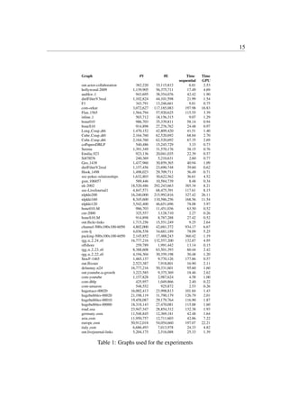
is frequently used in other studies. The first four columns of Table 1 lists the names,
number of vertices, number of edges, and sequential running time in seconds respec-
tively of the chosen graphs. The graphs are ordered by decreasing average vertex

14. 14
degree.
Our first set of experiments was performed to test the effect of changing the thresh-
old value used in Algorithm 1 for determining when an iteration of the modularity
optimization should end. As explained in Section 4 we use a larger threshold value
tbin when the graph size is above a predetermined limit and a smaller one tfinal when
it is below this limit. Similar to what was done in [16] this limit was set to 100, 000
vertices. We ran the algorithm with all combinations of threshold values (tbin, tfinal)
on the form (10k
, 10l
) where k varied from -1 to -4 and l from -3 to -7.
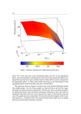
Figure 1 shows the average modularity over all graphs for each pair of values for
thfinal and thbin compared to the modularity given by the sequential algorithm. As
can be seen from the figure the relative modularity of the GPU algorithm decreases
when the thresholds increases. Still, the average modularity of the GPU algorithm is
never more than 2% lower than that given by the sequential algorithm. In Figure 2 we
show the relative speedup compared to the best speedup that was obtained when the
threshold values were varied. These numbers were obtained by first computing the best
speedup for each graph across all possible threshold configurations. For each threshold
configuration we then computed the relative distance from the best speedup for each
graph. Finally, we plot the average of these numbers for each threshold configuration.
It is clear from Figure 2 that the speedup is critically dependent on the value of
thbin, with higher values giving better speedup. However, this must be compared to
the corresponding decrease in modularity. Based on these observations we chose to
use a value of 10−6
for thfinal and 10−2
for thbin. With these choices we still have an
average modularity of over 99% compared to the sequential algorithm and an average
speedup of about 63% compared to the best one. The fifth column of Table 1 shows the
running time of the GPU algorithm using these parameters. The speedup of the GPU
algorithm relative to the sequential one is plotted in Figure 3. The speedup ranges from
approximately 2.7 up to 312 with an average of 41.7. However, these results depend on
using a higher value for thbin in the GPU algorithm. This value can also be used in the
sequential algorithm. In Figure 4 we show the speedup when the sequential algorithm
has been modified in this way.
The effect of doing this is that the running time of the sequential algorithm de-
creases significantly giving an average speedup of 7.3 compared to the original one.
The average modularity of the final solution only drops by a factor of 0.13% compared
to that of the original algorithm. The obtained speedup of the GPU algorithm is now
in the range from just over 1 up to 27 with an average of 6.7.
Next, we consider how the time is spent in the GPU algorithm. In figures 5 and 6
we show the breakdown of the running time over the different stages for the road usa
and nlpkkt200 graphs respectively. For each stage the time is further divided into the
time spent in the modularity optimization phase and in the aggregation phase.
Figure 5 gives the typical behaviour we experienced, with the first stage being the
most time consuming followed by a tail of less expensive stages. On a few graphs
this tail could go on up to a few hundred stages. On average the algorithm spends

15. 15
Graph #V #E Time Time
sequential GPU
out.actor-collaboration 382,220 33,115,812 6.81 2.53
hollywood-2009 1,139,905 56,375,711 17.49 4.69
audikw 1 943,695 38,354,076 42.42 1.90
dielFilterV3real 1,102,824 44,101,598 21.99 1.54
F1 343,791 13,246,661 9.81 0.75
com-orkut 3,072,627 117,185,083 197.98 16.83
Flan 1565 1,564,794 57,920,625 115.55 3.39
inline 1 503,712 18,156,315 9.07 1.29
bone010 986,703 35,339,811 58.14 0.94
boneS10 914,898 27,276,762 24.48 0.97
Long Coup dt6 1,470,152 42,809,420 41.51 1.40
Cube Coup dt0 2,164,760 62,520,692 68.84 2.70
Cube Coup dt6 2,164,760 62,520,692 67.35 2.69
coPapersDBLP 540,486 15,245,729 3.33 0.73
Serena 1,391,349 31,570,176 38.15 0.76
Emilia 923 923,136 20,041,035 22.39 0.57
Si87H76 240,369 5,210,631 2.60 0.77
Geo 1438 1,437,960 30,859,365 40.94 1.09
dielFilterV2real 1,157,456 23,690,748 39.60 0.62
Hook 1498 1,498,023 29,709,711 36.49 0.71
soc-pokec-relationships 1,632,803 30,622,562 36.61 4.52
gsm 106857 589,446 10,584,739 8.48 0.34
uk-2002 18,520,486 292,243,663 385.34 8.21
soc-LiveJournal1 4,847,571 68,475,391 117.61 8.15
nlpkkt200 16,240,000 215,992,816 327.42 26.11
nlpkkt160 8,345,600 110,586,256 168.56 11.54
nlpkkt120 3,542,400 46,651,696 78.08 3.97
bone010 M 986,703 11,451,036 63.50 0.52
cnr-2000 325,557 3,128,710 2.27 0.26
boneS10 M 914,898 8,787,288 27.42 0.52
out.flickr-links 1,715,256 15,551,249 9.25 2.64
channel-500x100x100-b050 4,802,000 42,681,372 934.17 6.67
com-lj 4,036,538 34,681,189 78.09 5.25
packing-500x100x100-b050 2,145,852 17,488,243 360.42 1.19
rgg n 2 24 s0 16,777,216 132,557,200 132.87 4.95
offshore 259,789 1,991,442 13.14 0.15
rgg n 2 23 s0 8,388,608 63,501,393 60.44 2.42
rgg n 2 22 s0 4,194,304 30,359,198 30.48 1.20
StocF-1465 1,465,137 9,770,126 177.86 0.57
out.flixster 2,523,387 7,918,801 16.90 2.11
delaunay n24 16,777,216 50,331,601 95.60 1.60
out.youtube-u-growth 3,223,585 9,375,369 18.46 2.62
com-youtube 1,157,828 2,987,624 4.58 1.00
com-dblp 425,957 1,049,866 2.40 0.22
com-amazon 548,552 925,872 2.53 0.26
hugetrace-00020 16,002,413 23,998,813 101.84 1.43
hugebubbles-00020 21,198,119 31,790,179 126.79 2.01
hugebubbles-00010 19,458,087 29,179,764 116.90 1.87
hugebubbles-00000 18,318,143 27,470,081 115.88 1.60
road usa 23,947,347 28,854,312 132.38 1.93
germany osm 11,548,845 12,369,181 42.48 1.64
asia osm 11,950,757 12,711,603 42.86 7.22
europe osm 50,912,018 54,054,660 197.07 22.21
italy osm 6,686,493 7,013,978 24.33 4.82
out.livejournal-links 5,204,175 2,516,088 25.33 1.39
Table 1: Graphs used for the experiments

16. 16
10−6
10−4
10−4 10−3 10−2 10−1
98
99
t
h
f
i
n
a
l
thbin
M
odularity(%)
98 98.5 99 99.5
Figure 1: Relative modularity for different threshold values
about 70% of the total time in the optimization phase and 30% in the aggregation
phase. Thus the algorithm is spending most of the time in the optimization phase even
though this part has been more carefully tuned to utilize GPU resources compared to
the aggregation phase. It follows that further fine tuning of the load balance in the
aggregation phase would most likely only give a limited effect.
The behaviour shown in Figure 6 occurred only in the channel-500 graph and the
three nlpkkt graphs. For all of these graphs we observed that in the first few stages
the graph size did not decrease significantly. We then get a time consuming modular-
ity optimization phase where the largest remaining community is up to two orders of
magnitude larger than what was seen in the previous stages. Following this stage the
size of the graph decreases considerably. We note that this effect happens while we are
still using the tbin threshold value. We suspect that this effect might occur on graphs
that lack a natural initial community structure.

17. 17
10−6
10−4
10−4 10−3 10−2 10−1
50
100
t
h
f
i
n
a
l
thbin
Speedup(%)
40 50 60 70 80 90
Figure 2: Relative speedup for different threshold values
In shared memory implementations such as those in [16] and [21] a thread is re-
sponsible for determining the next community for several vertices in the modularity
optimization phase. Once a new community has been computed for a vertex, it is im-
mediately moved to it. In this way each thread has knowledge about the progress of
other threads through the shared memory. At the other end of the scale, a pure fine
grained implementation would compute the next community of each vertex only based
on the previous configuration and then move all vertices simultaneously. Our algorithm
operates somewhere in between these two models by updating the global community
information following the processing of the vertices in each bin. A natural question
is then how the algorithm is affected by this strategy. To test this we ran experiments
where we only updated the community information of each vertex at the end of each it-
eration in the optimization phase. We label this as the “relaxed” approach. The results
showed that the average difference in modularity was less than 0.13% between the two
strategies. However, the running time would in some cases increase by as much as a

18. 18
3
20
60
90
300o
u
t
.
a
c
t
o
r
-
c
o
l
l
a
b
o
r
a
t
i
o
n
h
o
l
l
y
w
o
o
d
-
2
0
0
9
a
u
d
i
k
w
1
d
i
e
l
F
i
l
t
e
r
V
3
r
e
a
l
F
1
c
o
m
-
o
r
k
u
t
F
l
a
n
1
5
6
5
i
n
l
i
n
e
1
b
o
n
e
0
1
0
b
o
n
e
S
1
0
L
o
n
g
C
o
u
p
d
t
6
C
u
b
e
C
o
u
p
d
t
0
C
u
b
e
C
o
u
p
d
t
6
c
o
P
a
p
e
r
s
D
B
L
P
S
e
r
e
n
a
E
m
i
l
i
a
9
2
3
S
i
8
7
H
7
6
G
e
o
1
4
3
8
d
i
e
l
F
i
l
t
e
r
V
2
r
e
a
l
H
o
o
k
1
4
9
8
s
o
c
-
p
o
k
e
c
-
r
e
l
a
t
i
o
n
s
h
i
p
s
g
s
m
1
0
6
8
5
7
u
k
-
2
0
0
2
s
o
c
-
L
i
v
e
J
o
u
r
n
a
l
1
n
l
p
k
k
t
2
0
0
n
l
p
k
k
t
1
6
0
n
l
p
k
k
t
1
2
0
b
o
n
e
0
1
0
M
c
n
r
-
2
0
0
0
b
o
n
e
S
1
0
M
o
u
t
.
f
l
i
c
k
r
-
l
i
n
k
s
c
h
a
n
n
e
l
-
5
0
0
x
-
b
0
5
0
c
o
m
-
l
j
p
a
c
k
i
n
g
-
5
0
0
x
-
b
0
5
0
r
g
g
n
2
2
4
s
0
o
f
f
s
h
o
r
e
r
g
g
n
2
2
3
s
0
r
g
g
n
2
2
2
s
0
S
t
o
c
F
-
1
4
6
5
o
u
t
.
f
l
i
x
s
t
e
r
d
e
l
a
u
n
a
y
n
2
4
o
u
t
.
y
o
u
t
u
b
e
-
u
-
g
r
o
w
t
h
c
o
m
-
y
o
u
t
u
b
e
c
o
m
-
d
b
l
p
c
o
m
-
a
m
a
z
o
n
h
u
g
e
t
r
a
c
e
-
0
0
0
2
0
h
u
g
e
b
u
b
b
l
e
s
-
0
0
0
2
0
h
u
g
e
b
u
b
b
l
e
s
-
0
0
0
1
0
h
u
g
e
b
u
b
b
l
e
s
-
0
0
0
0
0
r
o
a
d
u
s
a
g
e
r
m
a
n
y
o
s
m
a
s
i
a
o
s
m
e
u
r
o
p
e
o
s
m
i
t
a
l
y
o
s
m
o
u
t
.
l
i
v
e
j
o
u
r
n
a
l
-
l
i
n
k
s
Speedup
Figure 3: Speedup of the GPU algorithm compared to the sequential algorithm
factor of ten when using the relaxed strategy. This was typically due to the optimiza-
tion phase immediately following the switch from tbin to tfinal. One other observed
difference was that the number of phases was in some instances significantly smaller
with the relaxed strategy, although this did not result in a clear trend in how the running
time was affected. In several cases the reduced number of iterations would be offset
by the algorithm spending more time in each iteration.
To see how our algorithm compares to other parallel implementations we have
compared our results with those of the parallel Louvain method (PLM) by Staudt and
Meyerhenke [21] using 32 threads. Our test sets contains four common graphs, coPa-
perDBLP, soc-LiveJournal1, europe osm, and uk-2002. On these graphs the average

19. 19
1
2
5
10
15
20
25
o
u
t
.
a
c
t
o
r
-
c
o
l
l
a
b
o
r
a
t
i
o
n
h
o
l
l
y
w
o
o
d
-
2
0
0
9
a
u
d
i
k
w
1
d
i
e
l
F
i
l
t
e
r
V
3
r
e
a
l
F
1
c
o
m
-
o
r
k
u
t
F
l
a
n
1
5
6
5
i
n
l
i
n
e
1
b
o
n
e
0
1
0
b
o
n
e
S
1
0
L
o
n
g
C
o
u
p
d
t
6
C
u
b
e
C
o
u
p
d
t
0
C
u
b
e
C
o
u
p
d
t
6
c
o
P
a
p
e
r
s
D
B
L
P
S
e
r
e
n
a
E
m
i
l
i
a
9
2
3
S
i
8
7
H
7
6
G
e
o
1
4
3
8
d
i
e
l
F
i
l
t
e
r
V
2
r
e
a
l
H
o
o
k
1
4
9
8
s
o
c
-
p
o
k
e
c
-
r
e
l
a
t
i
o
n
s
h
i
p
s
g
s
m
1
0
6
8
5
7
u
k
-
2
0
0
2
s
o
c
-
L
i
v
e
J
o
u
r
n
a
l
1
n
l
p
k
k
t
2
0
0
n
l
p
k
k
t
1
6
0
n
l
p
k
k
t
1
2
0
b
o
n
e
0
1
0
M
c
n
r
-
2
0
0
0
b
o
n
e
S
1
0
M
o
u
t
.
f
l
i
c
k
r
-
l
i
n
k
s
c
h
a
n
n
e
l
-
5
0
0
x
-
b
0
5
0
c
o
m
-
l
j
p
a
c
k
i
n
g
-
5
0
0
x
-
b
0
5
0
r
g
g
n
2
2
4
s
0
o
f
f
s
h
o
r
e
r
g
g
n
2
2
3
s
0
r
g
g
n
2
2
2
s
0
S
t
o
c
F
-
1
4
6
5
o
u
t
.
f
l
i
x
s
t
e
r
d
e
l
a
u
n
a
y
n
2
4
o
u
t
.
y
o
u
t
u
b
e
-
u
-
g
r
o
w
t
h
c
o
m
-
y
o
u
t
u
b
e
c
o
m
-
d
b
l
p
c
o
m
-
a
m
a
z
o
n
h
u
g
e
t
r
a
c
e
-
0
0
0
2
0
h
u
g
e
b
u
b
b
l
e
s
-
0
0
0
2
0
h
u
g
e
b
u
b
b
l
e
s
-
0
0
0
1
0
h
u
g
e
b
u
b
b
l
e
s
-
0
0
0
0
0
r
o
a
d
u
s
a
g
e
r
m
a
n
y
o
s
m
a
s
i
a
o
s
m
e
u
r
o
p
e
o
s
m
i
t
a
l
y
o
s
m
o
u
t
.
l
i
v
e
j
o
u
r
n
a
l
-
l
i
n
k
s
Speedup
Figure 4: Speedup compared to the adaptive sequential algorithm
modularity of the methods differed by less than 0.2%. The running time of coPaperD-
BLP in [21] was less than one second, while the other graphs all required more than 10
seconds each. On the three largest graphs our algorithm gave speedups ranging from a
factor of 1.3 to 4.6 with an average of 2.7 compared to [21].
We have also compared our results with the OpenMP code from [16]. Out of our
test set in Table 1 we were able to run 30 graphs on the computer equipped with two
Intel Xeon E5-2680 processors using 20 threads. For these tests we used NUMA aware
thread allocation and ”scatter mode” for thread pinning. Figure 7 gives the relative per-
formance of our GPU implementation compared to the OpenMP code on these graphs.

20. 20
1 2 3 4 5 6 7 8 9 10 11
0
0.1
0.2
0.3
0.4
0.5
0.6
0.7
0.8
0.9
1
1.1
Iteration
T
ime
road usa
Optimization
Aggregation
Figure 5: Time spent on the road usa graph
Our GPU implementation gave a speedup ranging from 1.1 to 27.0 with an average of
6.1. Note that both algorithms are using the same threshold values (10−2
, 10−6
) in the
modularity optimization phase.
To investigate what is causing this speedup, we have measured how much time both
algorithms are spending on the initial processing of each vertex in the first iteration of
the modularity optimization. In this part both algorithms are hashing exactly 2|E|
edges. The results show that the GPU code is on average 9 times faster than the code
from [16]. There are several possible explanations for this. The OpenMP code uses
locks in the preprocessing and the contraction phase, while the GPU code uses CAS
and atomic operations. Moreover, the GPU code is doing most of the hashing in shared
memory which is as fast as L1 cache. We also believe that the code from [16] could
execute faster if it employed better storage strategies for the hashing.
The GPU code has been profiled to see how it is utilizing the hardware resources
and how much parallelism is available. On UK-2002, on average 62.5% of the threads

21. 21
1 2 3 4 5 6 7 8 9 10 11 12 13 14 15
0
1
2
3
4
5
6
7
8
9
10
Iteration
T
ime
nlpkkt200
Optimization
Aggregation
Figure 6: Time spent on the nlpkkt200 graph
in a warp are active whenever the warp is selected for execution. The four schedulers
of each streaming multiprocessor has on average 3.4 eligible warps per cycle to choose
from for execution. Thus, despite the divergence introduced by varying vertex degrees
and memory latency, this indicate that we achieve sufficient parallelism to keep the
device occupied.
Finally, we note that the implementation in [20] reported a maximum processing
rate of 1.54 giga TEPS in the first modularity optimization phase when using a Blue
Gene/Q supercomputer with 8192 nodes and 524,288 threads. Our largest TEPS rate
was 0.225 giga TEPS obtained for the channel-500 graph. Thus the implementation
on the Blue Gene/Q gave less than a factor of 7 higher TEPS rate than our one using a
single GPU.

22. 22
1
5
10
20
30
h
o
l
l
y
w
o
o
d
-
2
0
0
9
a
u
d
i
k
w
1
d
i
e
l
F
i
l
t
e
r
V
3
r
e
a
l
F
1
F
l
a
n
1
5
6
5
i
n
l
i
n
e
1
b
o
n
e
0
1
0
b
o
n
e
S
1
0
L
o
n
g
C
o
u
p
d
t
6
C
u
b
e
C
o
u
p
d
t
0
C
u
b
e
C
o
u
p
d
t
6
c
o
P
a
p
e
r
s
D
B
L
P
E
m
i
l
i
a
9
2
3
G
e
o
1
4
3
8
d
i
e
l
F
i
l
t
e
r
V
2
r
e
a
l
H
o
o
k
1
4
9
8
g
s
m
1
0
6
8
5
7
u
k
-
2
0
0
2
s
o
c
-
L
i
v
e
J
o
u
r
n
a
l
1
c
h
a
n
n
e
l
-
5
0
0
x
-
b
0
5
0
p
a
c
k
i
n
g
-
5
0
0
x
-
b
0
5
0
r
g
g
n
2
2
4
s
0
o
f
f
s
h
o
r
e
r
g
g
n
2
2
3
s
0
r
g
g
n
2
2
2
s
0
S
t
o
c
F
-
1
4
6
5
a
s
i
a
o
s
m
e
u
r
o
p
e
o
s
m
i
t
a
l
y
o
s
m
Speedup
Figure 7: Speedup of the GPU implementation compared to [16]
6 Conclusion
We have developed and implemented the first truly scalable GPU version based on the
Louvain method. This is also the first implementation that parallelizes and load bal-
ances the access to individual edges. In this way our implementation can efficiently
handle nodes of highly varying degrees. Through a number of experiments we have
shown that it obtains solutions with modularity on par with the sequential algorithm.
In terms of performance it consistently outperforms other shared memory implemen-
tations and also compares favourably to a parallel Louvain method running on a super-
computer, especially when comparing the cost of the machines.
The algorithm achieved an even load balance by scaling the number of threads as-

23. 23
signed to each vertex depending on its degree. We note that similar techniques have
been used to load balance GPU algorithms for graph coloring [8] and for basic sparse
linear algebra routines [14]. We believe that employing such techniques can have a
broad impact on making GPUs more relevant for sparse graph and matrix computa-
tions, including other community detection algorithms.
We note that the size of the current GPU memory can restrict the problems that
can be solved. Although the memory size of GPUs is expected to increase over time,
this could be mitigated by the use of unified virtual addressing (UVA) to acquire mem-
ory that can be shared between multiple processing units. However, accessing such
memory is expected to be slower than on-card memory. We believe that our algorithm
can also be used as a building block in a distributed memory implementation of the
Louvain method using multi-GPUs. This type of hardware is fairly common in large
scale computers. Currently more than 58% of the 500 most powerful computers in the
world have some kind of GPU co-processors from NVIDIA [22].
Using adaptive threshold values in the modularity optimization phase had a signif-
icant effect on the running time of both the sequential and our parallel algorithm. This
idea could have been expanded further to include even more threshold values for vary-
ing sizes of graphs. It would also have been possible to fine tune the implementation of
the aggregation phase to further speed up the processing. However, as this is currently
not the most time consuming part, the effect of doing this would most likely have been
limited.
Finally, we note that coarse grained approaches seem to consistently produce solu-
tions of high modularity even when using an initial random vertex partitioning. This
could be an indication that the tested graphs do not have a clearly defined community
structure or that the algorithm fails to identify communities smaller than a network
dependent parameter [11].
References
[1] Vincent D. Blondel, Jean-Loup Guillaume, Renaud Lambiotte, and Etienne
Lefebvre. Fast unfolding of community hierarchies in large networks. CoRR,
abs/0803.0476, 2008.
[2] Ulrik Brandes, Daniel Delling, Marco Gaertler, Robert Görke, Martin Hoefer,
Zoran Nikoloski, and Dorothea Wagner. On modularity clustering. IEEE Trans.
Knowl. Data Eng., 20(2):172–188, 2008.
[3] Ümit V. Çatalyürek, Cevdet Aykanat, and Bora Uçar. On two-dimensional sparse
matrix partitioning: Models, methods, and a recipe. SIAM J. Scientific Comput-
ing, 32(2):656–683, 2010.
[4] Chun Yew Cheong, Huynh Phung Huynh, David Lo, and Rick Siow Mong Goh.
Hierarchical parallel algorithm for modularity-based community detection using

24. 24
GPUs. In Euro-Par 2013 Parallel Processing - 19th International Conference,
Aachen, Germany, August 26-30, 2013. Proceedings, volume 8097 of Lecture
Notes in Computer Science, pages 775–787. Springer, 2013.
[5] Thomas H. Cormen, Charles E. Leiserson, Ronald L. Rivest, and Clifford Stein.
Introduction to Algorithms. The MIT Press, third edition, 2009.
[6] D. Doyle D. Greene and P. Cunningham. Tracking the evolution of communities
in dynamic social networks. In Proceedings of the International Conference on
Advances in Social Networks Analysis and Mining, (ASONAM), pages 176–183,
2010.
[7] T. A. Davis and Y. Hu. The University of Florida sparse matrix collection. ACM
Trans. Math. Softw., 38(1):1–25, December 2011.
[8] Mehmet Deveci, Erik G. Boman, Karen D. Devine, and Sivasankaran Rajaman-
ickam. Parallel graph coloring for manycore architectures. In 2016 IEEE Inter-
national Parallel and Distributed Processing Symposium, IPDPS 2016, Chicago,
IL, USA, May 23-27, 2016, pages 892–901, 2016.
[9] Richard Forster. Louvain community detection with parallel heuristics on gpus.
In Proceedings of the 20th Jubilee IEEEInternational Conference on Intelligent
Engineering Systems, pages 227–232, 2016.
[10] S. Fortunato. Community detection in graphs. Physics Reports, 486(3-5):75–174,
2010.
[11] Santo Fortunato and Marc Barthelemy. Resolution limit in community detection.
PNAS, 104(1):36–41, 2007.
[12] konect network dataset - KONECT. http://konect.uni-koblenz.de, 2016.
[13] Jure Leskovec and Andrej Krevl. SNAP Datasets: Stanford large network dataset
collection. http://snap.stanford.edu/data, jun 2014.
[14] Weifeng Liu and Brian Vinter. A framework for general sparse matrix-matrix
multiplication on gpus and heterogeneous processors. Journal of Parallel and
Distributed Computing, 85:47–61, 2015.
[15] Yabing Liu, Krishna P. Gummadi, Balachander Krishnamurthy, and Alan Mis-
love. Analyzing facebook privacy settings: User expectations vs. reality. In
Proceedings of the 2011 ACM SIGCOMM Conference on Internet Measurement
Conference, IMC ’11, pages 61–70, New York, NY, USA, 2011. ACM.
[16] Hao Lu, Mahantesh Halappanavar, and Ananth Kalyanaraman. Parallel heuristics
for scalable community detection. Parallel Computing, 47:19–37, 2015.

25. 25
[17] D. Meunier, R. Lambiotte, A. Fornito, K. D. Ersche, and E. T. Bullmore. Hierar-
chical modularity in human brain functional networks. Frontiers in Neuroinfor-
matics, 37(3), 2010.
[18] M. E. J. Newman. Analysis of weighted networks. Phys. Rev. E, 70:056131,
2004.
[19] M. E. J. Newman and M. Girvan. Finding and evaluating community structure in
networks. Physical Review E, 69(2):026113, 2004.
[20] Xinyu Que, Fabio Checconi, Fabrizio Petrini, and John A. Gunnels. Scalable
community detection with the louvain algorithm. In 2015 IEEE International
Parallel and Distributed Processing Symposium, IPDPS 2015, Hyderabad, India,
May 25-29, 2015, pages 28–37. IEEE Computer Society, 2015.
[21] Christian L. Staudt and Henning Meyerhenke. Engineering parallel algorithms
for community detection in massive networks. IEEE Trans. Parallel Distrib. Syst.,
27(1):171–184, 2016.
[22] TOP500 Supercomputer Sites, list for November 2016. http://www.top500.org.
[23] Amanda L. Trauda, Peter J. Muchaa, and Mason A. Porter. Social structure
of facebook networks. Physica A: Statistical Mechanics and its Applications,
391(16):4165–4180, 2012.
[24] Brendan Vastenhouw and Rob H. Bisseling. A two-dimensional data distribution
method for parallel sparse matrix-vector multiplication. SIAM Review, 47(1):67–
95, 2005.
[25] Matthew L. Wallace, Yves Gingras, and Russell Duhon. A new approach for
detecting scientific specialties from raw cocitation networks. J. Am. Soc. Inf. Sci.
Technol., 60(2):240–246, 2009.
[26] Charith Wickramaarachchi, Marc Frı̂ncu, Patrick Small, and Viktor K. Prasanna.
Fast parallel algorithm for unfolding of communities in large graphs. In IEEE
High Performance Extreme Computing Conference, HPEC 2014, Waltham, MA,
USA, September 9-11, 2014, pages 1–6, 2014.
[27] Jianping Zeng and Hongfeng Yu. Parallel modularity-based community detection
on large-scale graphs. In 2015 IEEE International Conference on Cluster Com-
puting, CLUSTER 2015, Chicago, IL, USA, September 8-11, 2015, pages 1–10,
2015.
[28] XN. Zuo, R. Ehmke, M. Mennes, D. Imperati, FX. Castellanos, O. Sporns, and
MP. Milham. Network centrality in the human functional connectome. Cerebral
Cortex, 22:1862–1875, 2012.