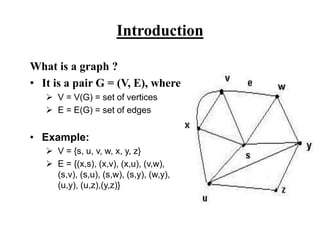
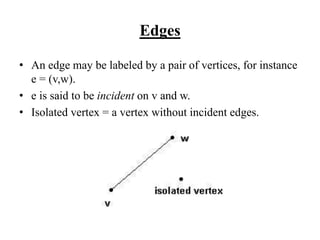
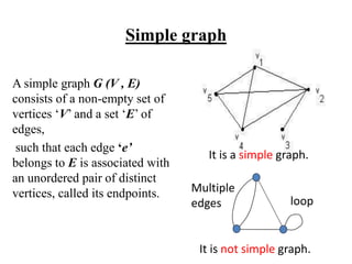
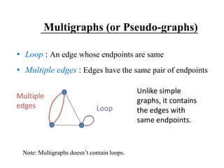
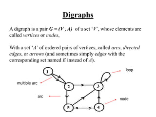
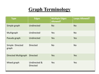
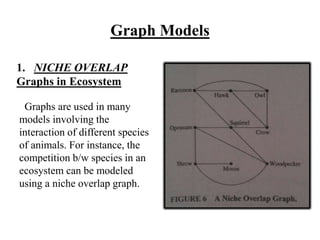
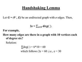
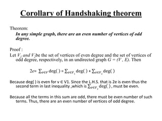
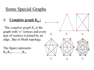
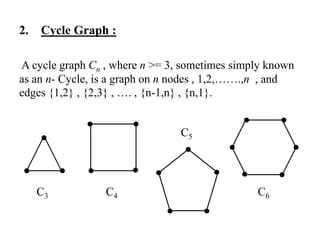
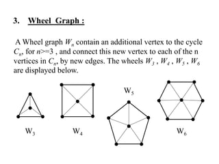
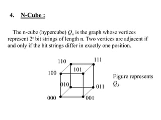
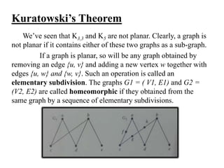
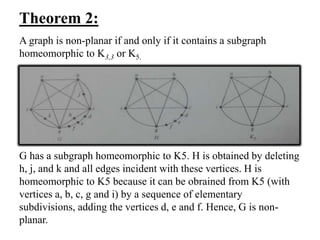
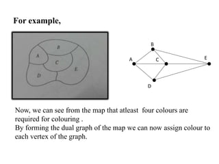
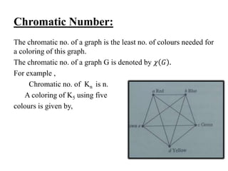
graph theory

CONTENTS
• 8.1 GRAPH & GRAPH MODELS
• 8.2 GRAPH TERMINOLOGIES
• 8.7 PLANAR GRAPH
• 8.8 GRAPH COLOURING

Introduction
What is a graph ?
• It is a pair G = (V, E), where
 V = V(G) = set of vertices
 E = E(G) = set of edges
• Example:
 V = {s, u, v, w, x, y, z}
 E = {(x,s), (x,v), (x,u), (v,w),
(s,v), (s,u), (s,w), (s,y), (w,y),
(u,y), (u,z),(y,z)}

Edges
• An edge may be labeled by a pair of vertices, for instance
e = (v,w).
• e is said to be incident on v and w.
• Isolated vertex = a vertex without incident edges.

A simple graph G (V , E)
consists of a non-empty set of
vertices ‘V’ and a set ‘E’ of
edges,
such that each edge ‘e’
belongs to E is associated with
an unordered pair of distinct
vertices, called its endpoints.
loop
Multiple
edges
It is not simple graph.
It is a simple graph.
Simple graph

Multigraphs (or Pseudo-graphs)
• Loop : An edge whose endpoints are same
• Multiple edges : Edges have the same pair of endpoints
Loop
Multiple
edges
Unlike simple
graphs, it contains
the edges with
same endpoints.
Note: Multigraphs doesn’t contain loops.

Digraphs
A digraph is a pair G = (V , A) of a set ‘V’, whose elements are
called vertices or nodes,
With a set ‘A’ of ordered pairs of vertices, called arcs, directed
edges, or arrows (and sometimes simply edges with the
corresponding set named E instead of A).
multiple arc
arc
node
loop

Graph Terminology
Type Edges Multiple Edges
Allowed?
Loops Allowed?
Simple graph Undirected No No
Multigraph Undirected Yes No
Pseudo graph Undirected Yes Yes
Simple Directed
graph
Directed No No
Directed Multigraph Directed Yes Yes
Mixed graph Undirected &
Directed
Yes Yes

Graph Models
1. NICHE OVERLAP
Graphs in Ecosystem
Graphs are used in many
models involving the
interaction of different species
of animals. For instance, the
competition b/w species in an
ecosystem can be modeled
using a niche overlap graph.

2. Round-Robin
Tournaments
A tournament where each
team plays each other team
exactly once is called a round-
robin tournament. Such
tournaments can be modeled
using directed graphs where
each team is represented by a
vertex.
Note: (a , b) is an edge if team
a beats team b and if the edge
is directed in the vertex then
that team is defeated by the
other one and vice-versa.

Degree of graph
The degree of a vertex in a simple graph, denoted by deg(v), is
the number of edges incident on it.
Degree also means number of adjacent vertices.
For a Node,
• The number of head endpoints adjacent to a node is called
the Indegree and it is denoted by deg- (v).
• The number of tail endpoints adjacent to a node is called
Outdegree and it is denoted by deg+ (v).

For example in the
digraph,
Out-deg(1) = 2
In-deg(1) = 0
Out-deg(2) = 2
In-deg(2) = 2
Out-deg(3) = 1
In-deg(3) = 4
And so on…….

Let G = (V , E) be an undirected graph with e edges. Then,
2e = 𝒗∈𝑽 𝒅𝒆𝒈( ).
For example,
How many edges are there in a graph with 10 vertices each
of degree six?
Solution:
deg( ) = 6*10 = 60
which follows 2e = 60 ,i.e., e = 30
Handshaking Lemma

Theorem:
In any simple graph, there are an even number of vertices of odd
degree.
Proof :
Let V1 and V2be the set of vertices of even degree and the set of vertices of
odd degree, respectively, in an undirected graph G = (V , E). Then
2e= 𝑣∈𝑉 deg = 𝑣∈𝑉1
deg + 𝑣∈𝑉2
deg
Because deg( ) is even for v ∈ V1. Since the L.H.S. that is 2e is even thus the
second term in last inequality ,which is 𝑣∈𝑉2
deg , must be even.
Because all the terms in this sum are odd, there must be even number of such
terms. Thus, there are an even number of vertices of odd degree.
Corollary of Handshaking theorem

Some Special Graphs
1. Complete graph Kn :
The complete graph Kn is the
graph with ‘n’ vertices and every
pair of vertices is joined by an
edge , like in Mesh topology.
The figure represents
K2,K3,………,K7.

2. Cycle Graph :
A cycle graph Cn , where n >= 3, sometimes simply known
as an n- Cycle, is a graph on n nodes , 1,2,…….,n , and
edges {1,2} , {2,3} , …. , {n-1,n} , {n,1}.
C3 C6
C5
C4

3. Wheel Graph :
A Wheel graph Wn contain an additional vertex to the cycle
Cn, for n>=3 , and connect this new vertex to each of the n
vertices in Cn, by new edges. The wheels W3 , W4 , W5 , W6
are displayed below.
W3 W6
W5
W4

4. N-Cube :
The n-cube (hypercube) Qn is the graph whose vertices
represent 2n bit strings of length n. Two vertices are adjacent if
and only if the bit strings differ in exactly one position.
100
000
101
001
110 111
010 011
Figure represents
Q3

Bipartite Graphs
• A bipartite graph G is a
graph such that
– V(G) = V(G1)  V(G2)
– |V(G1)| = m, |V(G2)| = n
– V(G1) V(G2) = Ø
No edges exist between any
two vertices in the same
subset V(Gk), k = 1,2
G1 G2

Complete Bipartite graph Km,n
A bipartite graph is the complete
bipartite graph Km,n if every vertex
in V(G1) is joined to a vertex in
V(G2) and conversely,
|V(G1)| = m , |V(G2)| = n

Bipartite Graphs in terms of
Graph Coloring
Theorem:
A simple graph is bipartite if and only if it is possible
to assign one of two different colors to each vertex of the
graph so that no two adjacent vertices are assigned the same
color.
K2 , 3
V2V1

Proof:
First, suppose that G = (V , E) is a simple graph. Then V = V1 U
V2, where V1 and V2 are disjoint sets and every edge in E connects a
vertex in V1 and a vertex in V2. If we assign one color to each vertex in
V1 and a second color to each vertex in V2, then no two adjacent
vertices are assigned the same color.
Now suppose that it is possible to assign colors to the vertices of
the graph using just two colors so that no two adjacent vertices are
assigned the same color. Let V1 be the set of vertices assigned one color
and V2 be the set of vertices assigned the other color. Then, V1 and V2
are disjoint and V = V1 U V2. Furthermore, every edge connects a
vertex in V1 and a vertex in V2 because no two adjacent vertices are
either both in V1 or both in V2.
Consequently, G is bipartite.

Applications of Special Types of Graphs
1. Job Assignments :
Suppose that there are m employees in a group and j different
jobs that need to be done where m<=j. Each employee is trained
to do one or more of these j jobs. We can use a graph to model
employee capabilities. We represent each employee by a vertex
and each job by a vertex. For each employee, we include an edge
from the vertex representing that employee to the vertices
representing all jobs the employee has been trained to do.

2. Local Area Network :
Various computers in a building, such as minicomputers and
personal computers, as well as peripheral devices such as printers and
plotters, can be where all devices are connected to a central control
device. A local network can be represented using a complete bipartite
graph K1,n. Messages are sent from device to device through the central
control device.
Other local area networks are based on a ring topology, where
each device is connected to exactly two others. Local area networks
with a ring topology are modeled using n-cycles, Cn. Messages are sent
from device to device around the cycle until the intended recipient of a
message is reached.

A graph is called planar if it can be drawn in the
plane without any edges crossing ,
(where a crossing of edges is the intersection of lines
or arcs representing them at a point other than their
common endpoint).
Such a drawing is called a planar representation
of the graph.
PLANAR GRAPHS :

Showing K4 is planar. Showing Q3 is non-planar.

Consider the problem of joining three houses to each of
three separate utilities as shown in the figure. Is it possible
to join these houses and utilities so that none of the
connections cross?
This problem can be modeled using the
complete bipartite graph K3,3 .

SOLUTION:
Any attempt to draw K3,3 in the plane with no edges crossing is
doomed. We now show why.
In any planar representation of K3,3 , the vertices 1 and 2 must be
connected to both 4 and 5. These four edges form a closed curve that
splits the plane into two regions, R1 and R2 , as shown in figure on
L.H.S.
Now, the vertex 3 is in either R1 or R2. When 3 is in R2, the inside of
the closed curve, the edges b/w 3 and 4 & b/w 3 and 5 separate R2 into
two subregions, R21 and R22, as shown in fig on R.H.S.
R2
R21
3
R22
1 5
24 4
1 5
2
R1 R1

Next, note that there is no way to place the final vertex 6 without
forcing a crossing.
• For if 6 is in R1, then the edge b/w 6 and 3 cannot be drawn
without a crossing.
• If 6 is in R21, then the edge b/w 2 and 6 cannot be drawn
without a crossing. If 6 is in R22, then the edge b/w 1 and 6
cannot be drawn without a crossing.

EULER’S FORMULA
Since, a planar representation of a graph splits the plane into regions,
including an unbounded region. For e.g.,
Acc. To Euler’s formula,
If G be a connected planar simple graph with e edges and v vertices.
Let r be the number of regions in a planar representation of G. Then
r = e – v + 2
and this no. will remain same in all planar representations of that
graph.
R2
R1
R5
R3
R4
R6

Proof:
First, we specify a planar representation of G. We will prove the
theorem by constructing a seq of sub-graphs G1,G2,……..,Ge = G,
successively adding an edge at each stage. This is done using the
following inductive definition.
• Base Case:
If e = 1, the graph consists of two vertex (i.e., v = 2) with a
single region surrounding it. So we have r = 1 – 2 + 2 which is
clearly right.
1 2
R1

Inductive step:
Now assume that rn = en – vn + 2. Let {an+1, bn+1} be the edge
that is added to Gn to obtain Gn+1. There are two possibilities:
1) Both an+1 and bn+1 are already in Gn. These two vertices must
be on the boundary of a common region R, or else it would be
impossible to add the edge {an+1, bn+1} to Gn w/o two edges
crossing (and Gn+1 is planar). In this case rn+1 = rn + 1, en+1
= en + 1 and vn+1 = vn. Thus, each side of the formula relating
the number of regions, edges and vertices increases by
exactly one, i.e.,
rn+1 = en+1 – vn+1 + 2

2) One of the two vertices of the new edge is not already in Gn.
Suppose that an+1 is in Gn but that bn+1 is not. Adding this new
edge does not produce any new regions, because bn+1 must be in a
region that has an+1 on its boundary. Consequently, rn+1 = rn.
Moreover, en+1 = en + 1 and vn+1 = vn + 1. Each side of the
formula relating the number of regions, edges and vertices
remains the same, so the formula is still true, i.e.,
rn+1 = en+1 – vn+1 + 2

Corollary of Euler’s Formula
C-1 :
If G is a connected planar simple graph with e edges and
v vertices, where v>=3, then e <=3v-6.
Proof:
Let a connected planar simple graph divides the plane
into r regions. Then the degree of each region is at least 3
because the graphs we discussed here are simple graphs.
In particular, note that the degree of the unbounded region
is at least 3 because there are at least three vertices in the
graph.

Note that the sum of the degrees of the regions is exactly twice
the no. of edges in the graph, because each edge occurs on the
boundary of a region exactly twice. Because each region has
degree greater than or equal to 3, it follows
2e = ∑ deg(R) >= 3r
Hence,
(2/3)e >= r
Using r = e – v + 2
(Euler’s theorem)
e – v + 2 <= (2/3) e
i.e., e/3 <= v - 2 which gives e <= 3v – 6.
Use this corollary to demonstrate that K5 is not planar.

But if we implies corollary 1 to prove for K3,3 is planar then it
follows the corollary but when we try to draw K3,3 then we found
that it is planar!
Corollary 2 :
If a connected planar simple graph has e edges and v
vertices with v>=3 and no circuits of length 3, then
e <= 2v – 4
for K3,3 e = 9 and 2v – 4 = 8 , shows that K3,3 is
non-planar.

Kuratowski’s Theorem
We’ve seen that K3,3 and K5 are not planar. Clearly, a graph is
not planar if it contains either of these two graphs as a sub-graph.
If a graph is planar, so will be any graph obtained by
removing an edge {u, v} and adding a new vertex w together with
edges {u, w} and {w, v}. Such an operation is called an
elementary subdivision. The graphs G1 = ( V1, E1) and G2 =
(V2, E2) are called homeomorphic if they obtained from the
same graph by a sequence of elementary subdivisions.

Theorem 2:
A graph is non-planar if and only if it contains a subgraph
homeomorphic to K3,3 or K5.
G has a subgraph homeomorphic to K5. H is obtained by deleting
h, j, and k and all edges incident with these vertices. H is
homeomorphic to K5 because it can be obrained from K5 (with
vertices a, b, c, g and i) by a sequence of elementary
subdivisions, adding the vertices d, e and f. Hence, G is non-
planar.

Graph Coloring :
A coloring of a simple graph is the assignment of a colour to
each vertex of the graph so that no two adjacent vertices are
assigned the same colour.
• First, make the dual graph of a map which u want to colour.
• Then, a graph can be coloured by assigning a different colour
to each of its vertices. However, one can find fewer no. of
colours than the vertices in the graph to colour it.

For example,
A E
B
C
D
Now, we can see from the map that atleast four colours are
required for colouring .
By forming the dual graph of the map we can now assign colour to
each vertex of the graph.

Chromatic Number:
The chromatic no. of a graph is the least no. of colours needed for
a coloring of this graph.
The chromatic no. of a graph G is denoted by 𝜒 𝐺 .
For example ,
Chromatic no. of Kn is n.
A coloring of K5 using five
colours is given by,

• χ(G) ≤ Δ(G) + 1
• Greedy Algorithm:
– Put the vertices of a graph in a sequence
– For each vertex in the sequence, assign it the lowest
indexed color not already assigned to adjacent vertices
• Not guaranteed to be optimal for every possible
sequence
• Guaranteed optimal for at least one sequence
Greedy Coloring (Algorithm)

Vertex 0 1 2 3 4 5
Color Yellow Yellow Yellow Green Green Green
Greedy Coloring Example

Vertex 0 3 1 4 2 5
Color Yellow Yellow Green Green Purple Purple
Greedy Coloring Example

Chromatic polynomial
• Polynomial which gives the number of ways of proper
coloring a graph using a given number of colors
• Ci = no. of ways to properly color a graph using exactly i
colors
• λ = total no of colors
• λ Ci = selecting I colors out of λ colors
• ΣCi
λ Ci = total number of ways a graph canbe properly
colored using λ or lesser no. of colors
Pn(λ) of G = ΣCi
λ Ci

K-chromatic Graph
Let G be a simple graph, and let PG(k) be the number of ways
of coloring the vertices of G with k colors in such a way that
no two adjacent vertices are assigned the same color. The
function PG(k) is called the chromatic polynomial of G.
As an example, consider complete graph K3 as shown in the
following figure.

• Then the top vertex can be assigned any of the k colors, the
left vertex can be assigned any k-1 colors, and right vertex can
be assigned any of the k-2 colors.
• The chromatic polynomial of K3 is therefore K(K -1)(K -2).
The extension of this immediately gives us the following
result.
• If G is the complete graph Kn, then Pn(K) = K(K - 1)(K - 2) . . .
(K - n +1).

• Each cell is a vertex
• Each integer label is a
“color”
• A vertex is adjacent to
another vertex if one of the
following hold:
– Same row
– Same column
– Same 3x3 grid
• Vertex-coloring solves
Sudoku
Applications: Sudoku

Given is a list of courses, and for each course the list of students
who want to register for it. The goal is to find a time slot for each
course (using as few slots as possible). If a student is registered
for courses p and q, add an edge between p and q.
If the resulting class can be colored with k = the number of
available slots (MWF 8 -9 , MWF 9 – 10 etc. are various slots),
then we can find a schedule that will allow the students to take all
the courses they want to.
Applications: Scheduling problem

Applications: Traffic signal design
Traffic signal design: At an intersection of roads, we want to install
traffic signal lights which will periodically switch between
green and red. The goal is to reduce the waiting time for cars
before they get green signal.
This problem can be modeled as a coloring problem. Each path
that crosses the intersection is a node. If two paths intersect
each other, there is an edge connecting them. Each color
represents a time slot at which the path gets a green light.

• Scheduling
• Register allocation
• VLSI channel routing
• Biological networks (Khor)
• Testing printed circuit boards (Garey, Johnson, & Hing)
Applications

graph theory

More Related Content

What's hot

Similar to graph theory

More from Shashank Singh

Recently uploaded

graph theory