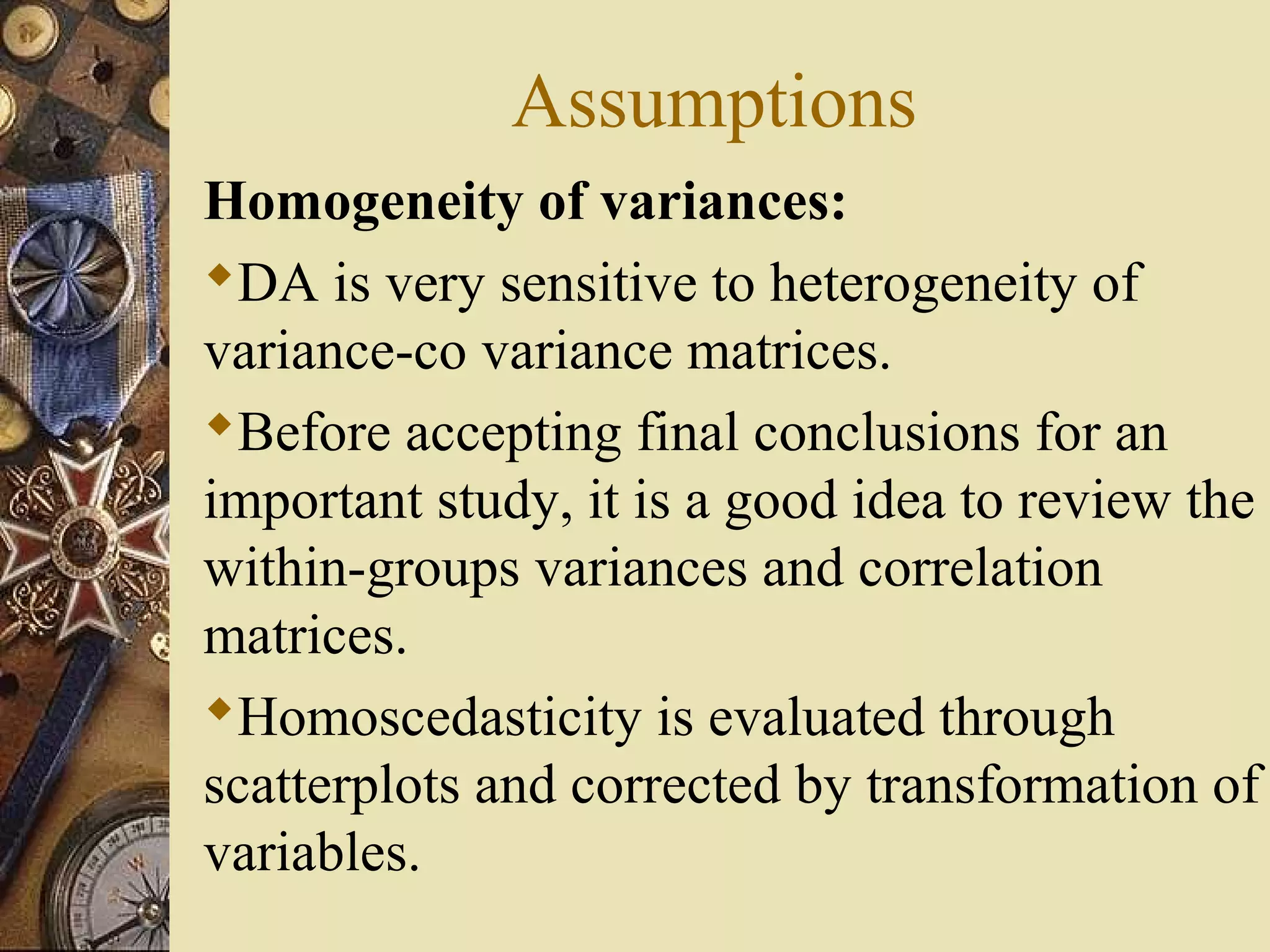
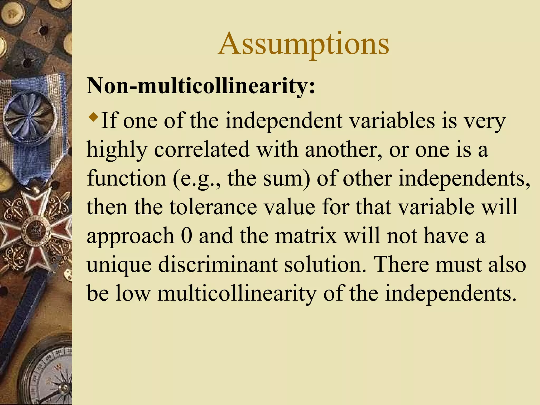
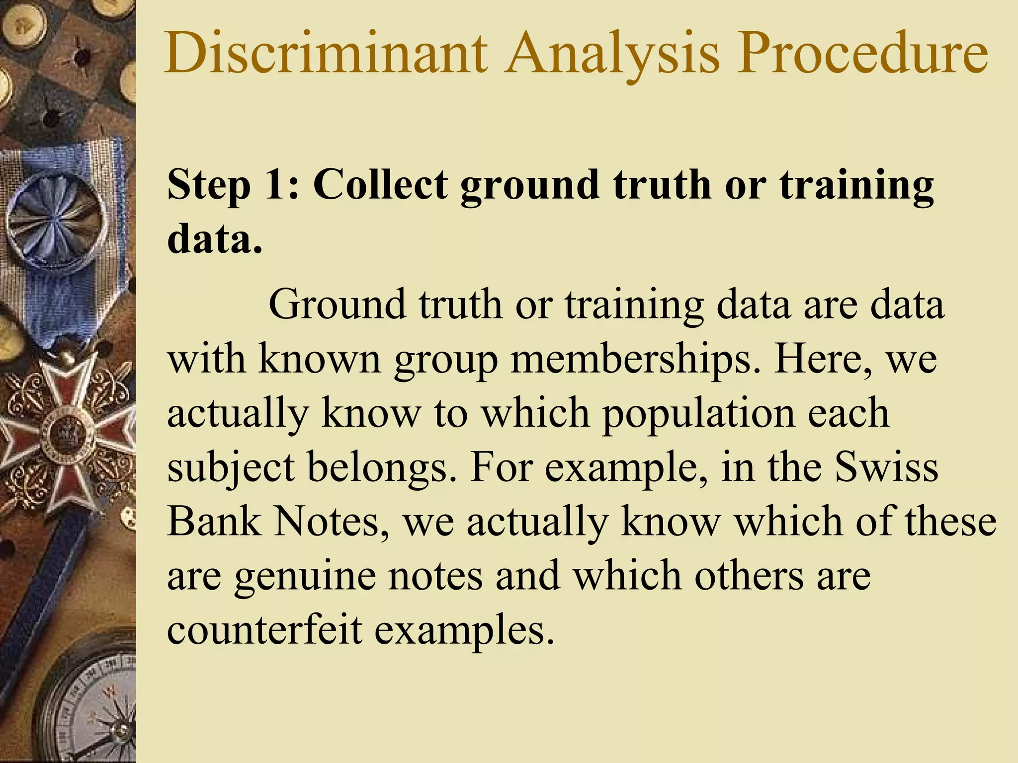
Discriminant analysis is a statistical technique used to classify cases into categories based on a set of predictor variables. It determines which continuous variables discriminate between two or more naturally occurring groups. For example, a researcher could use discriminant analysis to determine which fruit characteristics best predict whether a fruit will be eaten by birds, primates, or squirrels, based on data collected on various fruit properties from each animal group. Discriminant analysis involves estimating parameters, computing discriminant functions to classify new observations, and using cross-validation to estimate misclassification probabilities.

1. DiscriminantDiscriminant
AnalysisAnalysis

2. Discriminant Analysis
Discriminant analysis is a statistical
procedure which allows us to classify cases
in separate categories to which they belong
on the basis of a set of characteristic
independent variables called predictors or
discriminant variables

3. Discriminant Analysis
 Discriminant function analysis is used to
determine which continuous variables
discriminate between two or more
naturally occurring groups.
 For example, a researcher may want to
investigate which variables discriminate
between fruits eaten by (1) primates, (2)
birds, or (3) squirrels.

4. Discriminant Analysis
 For that purpose, the researcher could
collect data on numerous fruit
characteristics of those species eaten by
each of the animal groups. Most fruits will
naturally fall into one of the three
categories.
 Discriminant analysis could then be used
to determine which variables are the best
predictors of whether a fruit will be eaten
by birds, primates, or squirrels.

5. Discriminant Analysis & MANOVA
 Discriminant function analysis is
multivariate analysis of variance
(MANOVA) reversed.
 In MANOVA, the independent variables
are the groups and the dependent variables
are the predictors.
 In DA, the independent variables are the
predictors and the dependent variables are
the groups

6. Discriminant Function
Z = w1 X+ w2 Y
where,
X and Y are variables.
Sum of Squares between samples– SSb
Sum of Squares within samples – SSw
λ = (SSb/SSw)

7. Problem Description
 We have got a new cancer drug
* It works for some people.
* It makes other people worse.
 In order to discriminate between the two
groups we consider a dependent variable.
Here the variable is Gene expression of the
individual.

23. Assumptions
Sample size:
Unequal sample sizes are acceptable.
The sample size of the smallest group needs
to exceed the number of predictor variables.
 As a “rule of thumb”, the smallest sample
size should be at least 20 for a few (4 or 5)
predictors.
The maximum number of independent
variables is n - 2, where n is the sample size.

24. Assumptions
Normal distribution:
It is assumed that the data (for the variables)
represent a sample from a multivariate normal
distribution.
You can examine whether or not variables
are normally distributed with histograms of
frequency distributions. However, note that
violations of the normality assumption are not
"fatal" and the resultant significance test are
still reliable as long as non-normality is caused
by skewness and not outliers

25. Assumptions
Homogeneity of variances:
DA is very sensitive to heterogeneity of
variance-co variance matrices.
Before accepting final conclusions for an
important study, it is a good idea to review the
within-groups variances and correlation
matrices.
Homoscedasticity is evaluated through
scatterplots and corrected by transformation of
variables.

26. Assumptions
Outliers:
DA is highly sensitive to the inclusion of
outliers.
Run a test for univariate and multivariate
outliers for each group, and transform or
eliminate them. If one group in the study
contains extreme outliers that impact the
mean, they will also increase variability.
Overall significance tests are based on pooled
variances, that is, the average variance across
all groups.

27. Assumptions
Non-multicollinearity:
If one of the independent variables is very
highly correlated with another, or one is a
function (e.g., the sum) of other independents,
then the tolerance value for that variable will
approach 0 and the matrix will not have a
unique discriminant solution. There must also
be low multicollinearity of the independents.

28. Discriminant Analysis Procedure
Step 1: Collect ground truth or training
data.
Ground truth or training data are data
with known group memberships. Here, we
actually know to which population each
subject belongs. For example, in the Swiss
Bank Notes, we actually know which of these
are genuine notes and which others are
counterfeit examples.

29. Discriminant Analysis Procedure
Step 2: Prior Probabilities:
The prior probability pi represents the
expected portion of the community that
belongs to population πi. There are three
common choices:
1) Equal priors.
2) Arbitrary priors.
3) Estimated priors.

30. Discriminant Analysis Procedure
Step 3:
Use Bartlett’s test to determine if
variance-covariance matrices are
homogeneous for the two or more
populations involved. Result of this test will
determine whether to use Linear or Quadratic
Discriminant Analysis.
Case 1: Linear discriminant analysis is for
homogeneous variance-covariance matrices.
Case 2: Quadratic discriminant analysis is
used for heterogeneous variance-covariance
matrices

31. Discriminant Analysis Procedure
Step 4:
Estimate the parameters of the
conditional probability density functions
f ( X | πi ). Here, we shall make the following
standard assumptions:
*The data from group i has common mean vector μi
*The data from group i has common variance-
covariance matrix Σ.
*Independence: The subjects are independently
sampled.
*Normality: The data are multivariate normally
distributed.

32. Discriminant Analysis Procedure
Step 5:
Compute discriminant functions. This
is the rule for classification of the new object
into one of the known populations.
Step 6:
Use cross validation to estimate
misclassification probabilities.
Step 7:
Classify observations with unknown
group memberships

33. SPSSSPSS
VIDEOVIDEO