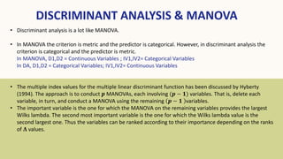
Discriminant analysis is a technique that is used by the researcher to analyze the research data when the criterion or the dependent variable is categorical and the predictor or the independent variable is the interval in nature. The term categorical variable means that the predictor variable is divided into a number of categories. DA is typically used when the groups are already defined prior to the study. The end result of DA is a model that can be used for the prediction of group memberships. This model allows us to understand the relationship between the set of selected variables and the observations. Furthermore, this model will enable one to assess the contributions of different variables.

1. DISCRIMINANT
ANALYSIS-I
Devendra Patil (AS_05)
M.Sc. Applied Statistics

2. INTRODUCTION
Discriminant analysis is a technique that is used by the researcher to
analyze the research data when the criterion or the dependent variable is
categorical and the predictor or the independent variable is the interval
in nature. The term categorical variable means that the predictor variable
is divided into a number of categories.
DA is typically used when the groups are already defined prior to the
prior to the study.
The end result of DA is a model that can be used for the prediction of
group memberships. This model allows us to understand the relationship
between the set of selected variables and the observations.
Furthermore, this model will enable one to assess the contributions of
different variables.

3. DISCRIMINANT ANALYSIS AND
BINARY LOGISTIC REGRESSION
Discriminant Analysis and Binary Logistic Regression
although they do the same thing same job but
discriminant is more powerful in comparison to logistic
because logistics is generally done with 0 and 1 case
yes or no case but discriminant analysis can take up
more than 2,3,4 also categories but larger too large
number of categories also is not very advisable.

4. ASSUMPTIONS OF
DISCRIMINANT
ANALYSIS
• Homogeneous within-group
variances.
• Multivariate normality within groups.
• No multi-collinearity.
• Prior probabilities.

5. HOMOGENEOUS WITHIN-GROUP VARIANCES.
Variances among group variables are the same across levels of predictors. It has been suggested,
however, that linear discriminant analysis be used when covariances are equal, and that quadratic
discriminant analysis may be used when covariances are not equal.
DA is very sensitive to the heterogeneity of variance-covariance matrices. Before accepting the final
conclusions for an important study, review the within-group variances and correlation matrices.
Homoscedasticity is evaluated through scatterplots and corrected by the transformation of variables.
The heterogeneity may arise due to the non-normality of data. Another one is due to large sample
since the significance probability becomes smaller even for almost homogeneous covariance matrices
if the sample size is large.
NO MULTI-COLLINEARITY.
Predictive power can decrease with an increased correlation between predictor variables.

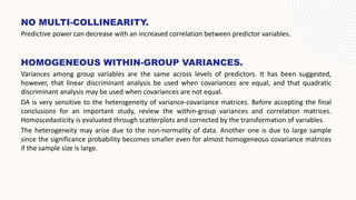
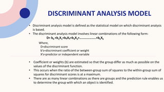
6. BOX’s M-Test
𝑯𝑶: 𝜮𝟏 = 𝜮𝟐=….= 𝜮𝑳
𝑯𝟏: 𝜮𝒍 ≠ 𝜮𝒎 for at least one pair of (l,m) is statistically different [ 𝒍 ≠ m]
Statistic D=(1-u)M
M= -2ln[ 𝒊=𝑙
𝑳
(
|𝑺𝒍|
|𝑺𝒑𝒐𝒐𝒍𝒆𝒅|
)
(𝒏𝒍−𝟏)
𝟐 ] (Log we used here for our convenience.)
u=[ 𝑙
1
(𝑛𝑙−1)
−
1
𝑙(𝑛𝑙−1)
] [
2𝑝2+3𝑝−1
6(𝑝+1)(𝐿−1)
]
Reject 𝑯𝒐 when D > 𝝌𝟐
𝜶,𝒗
D.F.= v
v =
1
2
p(p + 1)(L − 1)

7. PRIOR PROBABILITIES.
The prior probability is the probability of an observation coming from a particular group in a
simple random sample with replacement.
If the prior probabilities are the same for all three of the groups (also known as equal priors), then
the function is only based on the squared MAHALANOBIS distance.
MULTIVARIATE NORMALITY WITHIN GROUPS.
The independent variables should be multivariate normal; in other words, when all other
independent variables are held constant, the independent variable under examination should
have a normal distribution.
Mahalanobis procedure: a stepwise procedure used in discriminant analysis to maximize a
generalized measure of the distance between the two closest groups.

8. OBJECTIVES
• To find the linear combinations of variables that discriminate
between categories of dependent variables in the best possible
manner.
• To find out which independent variables are relatively better
in discriminating between groups.
• To determine the statistical significance of the discriminant
function and whether any statistical difference exists among
groups in terms of the predictor variable.
• To evaluate the accuracy of classification, i.e., the percentage
of customers that is able to classify correctly.

9. DISCRIMINANT ANALYSIS & MANOVA
• Discriminant analysis is a lot like MANOVA.
• In MANOVA the criterion is metric and the predictor is categorical. However, in discriminant analysis the
criterion is categorical and the predictor is metric.
In MANOVA, D1,D2 = Continuous Variables ; IV1,IV2= Categorical Variables
In DA, D1,D2 = Categorical Variables; IV1,IV2= Continuous Variables
• The multiple index values for the multiple linear discriminant function has been discussed by Hyberty
(1994). The approach is to conduct 𝒑 MANOVAs, each involving (𝒑 − 𝟏) variables. That is, delete each
variable, in turn, and conduct a MANOVA using the remaining 𝒑 − 𝟏 variables.
• The important variable is the one for which the MANOVA on the remaining variables provides the largest
Wilks lambda. The second most important variable is the one for which the Wilks lambda value is the
second largest one. Thus the variables can be ranked according to their importance depending on the ranks
of 𝚲 values.

10. 10

11. DISCRIMINANT ANALYSIS
The linear combination can be represented by D=b’X, where D is the discriminant
score of order (1 x n), b is a (p x 1)vector of discriminant weight and X is the
(n x p) data matrix.
In two groups of discriminant problems, the sample objects are classified with the help of a binary or
indicator variable with values zero and one. Now, corresponding to this binary variable the discriminant score D=b’X is
calculated using the data matrix X . This calculated discriminant score looks like the fitted multiple regression line when the
binary variable is considered as dependent one. In such situations, Y=b’X is a linear probability model where Y is the binary
variable and X is the matrix of the explanatory variables.
However, multiple regression analysis is not similar to discriminant analysis. The predictor variable in
multiple linear regression analysis is assumed to be normally distributed, whereas the binary variable in the discriminant
analysis does not follow any statistical distribution.
The explanatory variables in regression analysis do not follow any statistical distribution but in discriminant
analysis follow a multivariate normal distribution.
The objective of regression analysis is to predict response variables on the basis of predictors, whereas the
objective of discriminant analysis is to classify the sample objects with minimum classification error.

12. DISCRIMINANT ANALYSIS MODEL
• Discriminant analysis model is defined as the statistical model on which discriminant analysis
is based.
• The discriminant analysis model involves linear combinations of the following form:
D= b0 +b1X1+b₂X₂+b3X3+………………..+bkXk
Where,
D=discriminant score
b’s=discriminant coefficient or weight
X’s=predictor or independent variable
• Coefficient or weights (b) are estimated so that the group differ as much as possible on the
values of the discriminant function.
• This occurs when the ratio of the between-group sum of squares to the within-group sum of
squares for discriminant scores is at a maximum.
• There are as many linear combinations as there are groups and the prediction rule enables us
to determine the group with which an object is identified.

13. Canonical correlation: It measures the extent of association
between the discriminant score and the group.
Centroid: It is the mean value for the discriminant scores for a
particular group.
Classification matrix: It contains the number of correctly classified
and misclassified cases.
Hit Ratio: In the classification matrix, the sum of diagonal elements
divided by the total number of cases represents the hit ratio. It is the
percentage of cases correctly classified by discriminant analysis.
Discriminant function coefficients:
1)Discriminant function coefficients (unstandardized) are the
multipliers of variables. When the variables are in the original units
of measurement.
2)They are the discriminant function coefficients that are used as the
multipliers when the variables have been standardized to a mean 0
and variance 1.

14. Discriminant scores: The unstandardized coefficients are multiplied by the
values of the variables. These products are summed and added to the
constant term to obtain the discriminant scores.
Eigenvalue: For each discriminant function, the eigenvalue is the ratio of
between-group to within-group sums of squares.
• Wilks’ Lambda is the ratio of within-group sums of squares to the total sums
of squares. This is the proportion of the total variance in the discriminant
scores not explained by differences among groups.
• Wilks’ lambda takes a value between 0 and 1 and the lower the value of Wilks’
lambda, the higher the significance of the discriminant function as the
decrease in error of classification leads to a decrease in the amount of
variance.

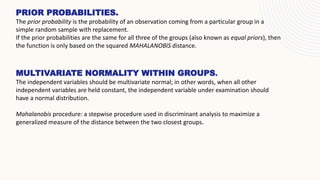
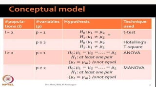
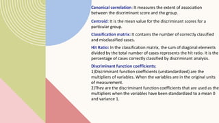
15. Let 𝑿𝒍 𝒏𝒍 × 𝒑 be the 𝑙-th data matrix [𝒍 = 𝟏, 𝟐, … , 𝒌] from 𝑵𝒑 𝝁𝒍, 𝜮𝒍 .
Assume that 𝜮𝟏 = 𝜮𝟐 = ⋯ = 𝜮𝒌. If 𝑿𝒍 = 𝑿𝟏𝒍𝑿𝟐𝒍 ⋯ 𝑿𝒑𝒍
′
be the data vector
and 𝒇𝒍 𝑿𝒍 be the density function of 𝑿𝒍, then the objective of the
discriminant analysis is to identify the 𝒇𝒍 𝑿𝒍 of an object on the basis of the
values of 𝒑 variables of 𝑿. The identification is done in such a way that the
error of identification is minimum.
Let us explain the technique by an example. Consider that a doctor needs to
examine many patients to diagnose their diseases. Different patients are
suffering from different diseases and the symptoms of the diseases are also
different. The symptoms help the doctor to diagnose the disease correctly
which in turn makes the patient cure. The treatment of the patient
becomes easier if the diagnosis of the disease is made correctly.
Justification of Discriminant Analysis and Selection of
Variables

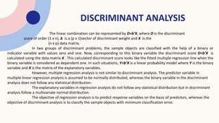
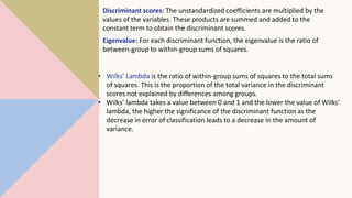
16. 𝑫 = 𝜷𝟎 + 𝜷𝟏𝒙𝟏 + 𝜷𝟐𝒙𝟐 + ⋯ + 𝜷𝒑𝒙𝒑
Let us consider that the total sample objects of size 𝒏 are to be divided into two
groups of sizes 𝒏𝟏 and 𝒏𝟐 such that 𝒏 = 𝒏𝟏 + 𝒏𝟐. Let us assume that 𝒍-th [𝒍 = 𝟏, 𝟐]
group of sample observations have the p.d.f. 𝒇𝒍(𝒙), where 𝒍-th population has mean
vector 𝝁𝒍. Now, if it is observed that the null hypothesis 𝑯𝟎: 𝝁𝟏 = 𝝁𝟐 is rejected, the
discriminant analysis can be performed.
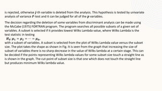
The rejection of 𝑯𝟎: 𝝁𝟏 = 𝝁𝟐 = ⋯ = 𝝁𝒌 does not mean that the means of 𝒋-th variable [𝒋 =
𝟏, 𝟐, … , 𝒑] for all 𝒌 samples are heterogeneous. If some of the means, assume that the means of
𝒑𝟏 < 𝒑 variables, are homogeneous, the above hypothesis may be rejected and decision will be
made in favor of discriminant analysis. However, the homogeneity in the variables in 𝒌 groups
has nothing to contribute to discriminate among groups.
Thus, even if the hypothesis of equality of group means is rejected, it needs a decision regarding
the inclusion of variables for discriminant analysis. Let 𝝁𝒍𝒋(𝒍 = 𝟏, 𝟐, … , 𝒌; 𝒋 = 𝟏, 𝟐, … , 𝒑) be the
mean of 𝑗-th variable of 𝑙-th sample. The 𝑗-th variable should be included in the analysis if the
null hypothesis
𝑯𝟎: 𝝁𝟏𝒋 = 𝝁𝟐𝒋 = ⋯ = 𝝁𝒌𝒋

17. is rejected, otherwise 𝒋-th variable is deleted from the analysis. This hypothesis is tested by univariate
analysis of variance 𝑭-test and it can be judged for all of the 𝒑 variables.
The decision regarding the deletion of some variables from discriminant analysis can be made using
the McCabe (1975) FORTRAN program. The program searches all possible subsets of a given set of
variables. A subset is selected if it provides lowest Wilks Lambda value, where Wilks Lambda is the
test statistic in testing
𝑯𝟎: 𝝁𝟏 = 𝝁𝟐 = ⋯ = 𝝁𝒌,
with a subset of variables. A subset is selected from the plot of Wilks Lambda value versus the subset
size. The plot takes the shape as shown in Fig. It is seen from the graph that increasing the size of
subset of variables there is no sharp decrease in the value of Wilks lambda at a certain stage. This can
be decided if the points representing Wilks lambda values for some subset size touch a straight line as
is shown in the graph. The cut point of subset size is that one which does not touch the straight line
but produces minimum Wilks lambda value.

19. The correlation coefficient of 𝑫 values and 𝒙𝒋(𝒋 = 𝟏, 𝟐, … , 𝒑) values. This correlation is used to
measure the contribution of 𝒋-th variable in discriminating the groups. The most contributing
variable is one for which the above-mentioned correlation coefficient is maximum.
If any pair of variables are highly correlated, which one has more discriminating power when both of
these are highly correlated with 𝑫. The amount of correlation of 𝑫 and 𝒙𝒋 and the sign of correlation
coefficient will be affected if 𝒙𝒋 and 𝒙𝒋′ 𝒋 ≠ 𝒋′
are highly correlated. thus if 𝒙𝒋 and 𝒙𝒋′ are
correlated, their correlation with 𝑫 will not provide any fruitful information about discriminating
power of the variable.
To avoid this, pooled within-groups correlation of all variables for all sample points are studied. If any
pair of variables is highly correlated, these are linearly related. The linear relationship may exist
among different variables. Let 𝒙𝒋 is linearly related with other 𝒙𝒋′ 's 𝒋′
≠ 𝒋 = 𝟏, 𝟐, … , 𝒑 and the
multiple correlation coefficient of 𝒋-th variable with other variables be 𝑹𝒋. Then 𝟏 − 𝑹𝒋
𝟐
is known
as tolerance. Now, if tolerance of any of the 𝒋-th variable is small, the inclusion of that variable in
discriminant analysis will not be fruitful.

20. THANK YOU