jitenderanduat@gmail.com

1. Canonical Correlation
Analysis
Presented by:
Jitendra Kumar
ID No. DFK 1303
Department of Fisheries Resources and
Management

2. Canonical Correlation?
Interrelationships between sets of
multiple independent variables
and multiple dependent
measures (quantify the strength
of the relationship)

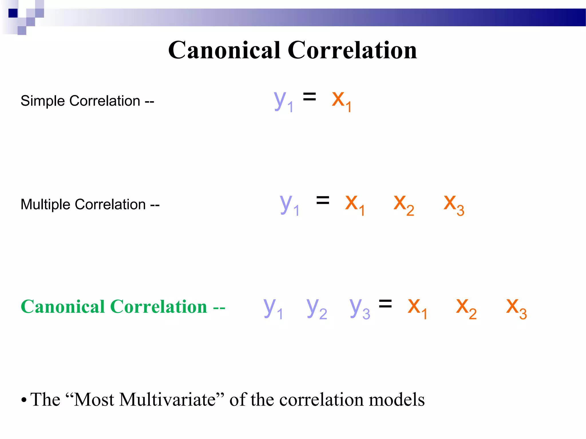
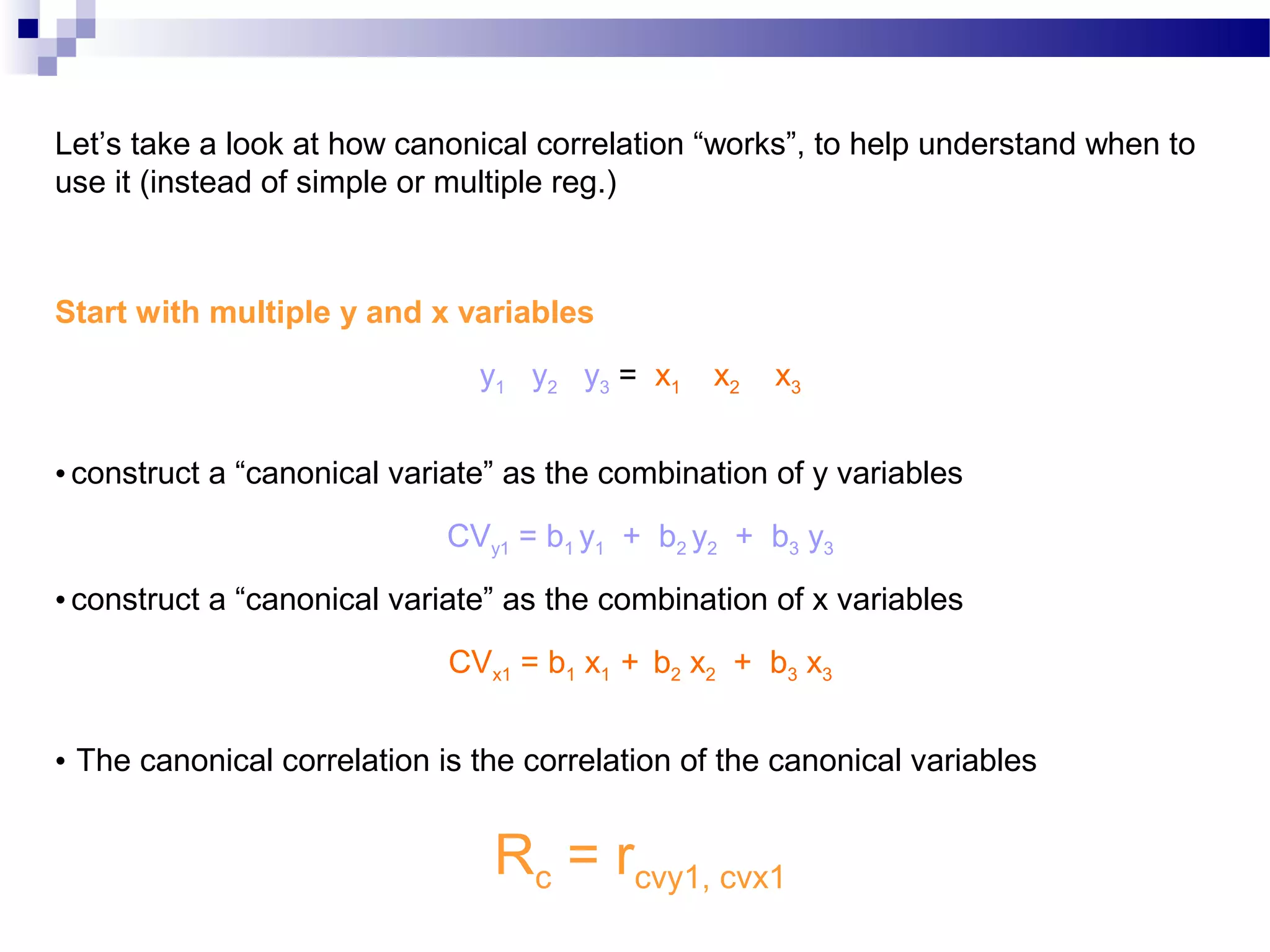
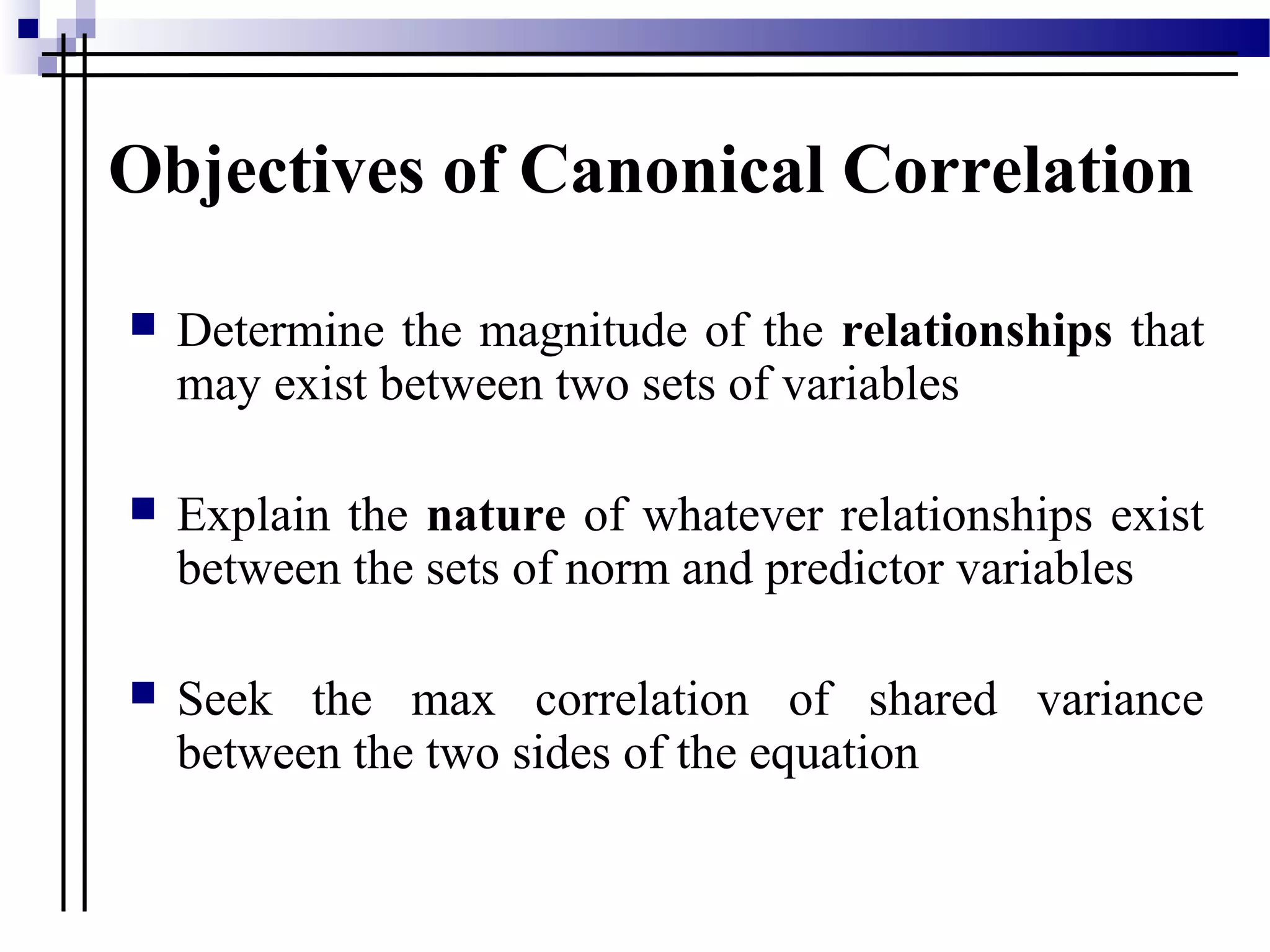
3. What is CCA?
 “Commonly used by researchers trying to
understand the relationship between
community composition and environmental
factors.”
Or, more generally, comparing/testing one
multivariate dataset against a second one.

4.  CCA was developed by H. Hotelling (1936).
 Although being a standard tool in statistical analysis
 where canonical correlation has been used for example
in economics, medical studies, meteorology and even in
classification of malt whisky,
 it is surprisingly unknown in the fields of learning and
signal processing.

5. Canonical Correlation
Simple Correlation -- y1 = x1
Multiple Correlation -- y1 = x1 x2 x3
Canonical Correlation -- y1 y2 y3 = x1 x2 x3
•The “Most Multivariate” of the correlation models

6. Let’s take a look at how canonical correlation “works”, to help understand when to
use it (instead of simple or multiple reg.)
Start with multiple y and x variables
y1 y2 y3 = x1 x2 x3
• construct a “canonical variate” as the combination of y variables
CVy1 = b1 y1 + b2 y2 + b3 y3
• construct a “canonical variate” as the combination of x variables
CVx1 = b1 x1 + b2 x2 + b3 x3
• The canonical correlation is the correlation of the canonical variables
Rc = rcvy1, cvx1

7. Objectives of Canonical Correlation
 Determine the magnitude of the relationships that
may exist between two sets of variables
 Explain the nature of whatever relationships exist
between the sets of norm and predictor variables
 Seek the max correlation of shared variance
between the two sides of the equation

8. CCA Purpose?
To incorporate environmental data into the
ordination so that a better final ordination
diagram can be created

9. What’s needed
1. Dependent matrix – contains data to be ordinate, usually
composed of population estimates for a bunch of species)
2. Environmental matrix – describes environmental
conditions. Must contain the same number of rows
(observations) as the species data, but must have fewer
columns than the number of observations.

10. The difference between CCA and ordinary correlation
analysis
 Ordinary correlation analysis is dependent on the coordinate system in
which the variables are described.
This means that even if there is a very strong linear relationship between two
multidimensional signals, this relationship may not be visible in a ordinary
correlation analysis if one coordinate system is used, while in another
coordinate system this linear relationship would give a very high
correlation.
 CCA finds the coordinate system that is optimal for correlation analysis,
and the eigenvectors of equation 4 defines this coordinate system.

11. Limitations
 Rc reflects only the variance shared by the linear
composites, not the variances extracted from the
variables
 Canonical weights are subject to a great deal of
instability
 Interpretation difficult because rotation is not
possible
 Precise statistics have not been developed to
interpret canonical analysis

12. Analyzing Relationships with Canonical Correlation
 Stage 1: Objectives of Canonical
Correlation Analysis
 Determine relationships among sets of variables
 Achieve maximal correlation
 Explain nature of relationships among sets of variables
 Stage 2: Designing a Canonical
Correlation Analysis
 Sample size
 Stage 3: Assumptions in Canonical
Correlation

13. Analyzing Relationships with Canonical Correlation (Cont.)
 Stage 4: Deriving the Canonical Functions
and Assessing Overall Fit
Deriving Canonical Variates (Functions)
 Each of the pairs of variates is orthogonal and independent of
all other variates derived from the same set of data
Which Canonical Functions Should Be Interpreted?
 Level of Significance
 Magnitude of the Canonical Relationships
 Redundancy Measure of Shared Variance

14. Analyzing Relationships with Canonical Correlation (Cont.)
 Stage 5: Interpreting the Canonical Variate
Canonical Weights (standardized coefficients)
Canonical Loadings (structure correlations)
Canonical Cross-Loadings
Which Interpretation Approach to Use
 Stage 6: Validation and Diagnosis