1. The University of Newcastle
Brief Review of Discrete-Time Systems
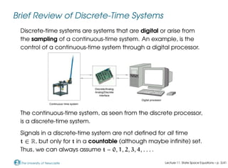
Discrete-time systems are systems that are digital or arise from
the sampling of a continuous-time system. An example, is the
control of a continuous-time system through a digital processor.
Discrete/Analog
Analog/Discrete
Interface
Continuous−time system
Digital processor
0000
0000
0000
0000
0000
0000
1111
1111
1111
1111
1111
1111
The continuous-time system, as seen from the discrete processor,
is a discrete-time system.
Signals in a discrete-time system are not defined for all time
t ∈ R, but only for t in a countable (although maybe infinite) set.
Thus, we can always assume t = 0, 1, 2, 3, 4, . . . .
Lecture 11: State Space Equations – p. 3/41
2. The University of Newcastle
Brief Review of Discrete-Time Systems
Define the impulse sequence δ[k] as
δ[k − m] =
1 if k = m
0 if k 6= m
where k and m are integers.
m + 1
m
k
δ[k − m]
In the discrete-time case impulses are easy to implement
physically, in contrast to the continuous-time case.
A sequence u[k] can be represented by means of the series
u[k] =
∞
X
m=−∞
u[m] δ[k − m] .
Lecture 11: State Space Equations – p. 4/41
3. The University of Newcastle
Brief Review of Discrete-Time Systems
Let g[k − m] denote the response of a causal, discrete-time
linear time-invariant (LTI) system to a unit impulse applied at the
instant m.
m + 1
m
k
G
g[k − m]
k
m
δ[k − m]
Then the output of the system to an arbitrary input sequence
u[k] is given the discrete convolution
y[k] =
∞
X
k=0
g[k − m] u[m]
=
∞
X
k=0
g[m] u[k − m].
Lecture 11: State Space Equations – p. 5/41
9. The University of Newcastle
Brief Review of Discrete-Time Systems
The equation
Y(z) = G(z)U(z)
is the discrete counterpart of the transfer function
representation Y(s) = G(s)U(s) for continuous-time systems.
The function G(z) is the z-transform of the impulse response
sequence g[k] and is called the discrete transfer function.
Both the discrete convolution and transfer function describe
the system assuming zero initial conditions.
Lecture 11: State Space Equations – p. 7/41
10. The University of Newcastle
Brief Review of Discrete-Time Systems
Example. Consider the unit-sampling-time delay system defined
by
y[k] = u[k − 1].
The output equals the input delayed by one sampling period. Its
impulse response sequence is g[k] = δ[k − 1] and its discrete
transfer function is
G(z) = Z{δ[k − 1]} = z−1
=
1
z
.
It is a rational function of z. Note that every continuous-time
system involving a time-delay is a distributed system. This is not so
in discrete-time systems.
Lecture 11: State Space Equations – p. 8/41
11. The University of Newcastle
Brief Review of Discrete-Time Systems
Example. Consider the discrete-time system of the block
diagram below.
k
c c
-
- -
6
-
Gain
a
y[k]
z−1
Unit time delay
u[k]
r[k]
+
+
If the unit-sampling-time delay is replaced by its discrete transfer
function z−1
, then the discrete transfer function from r to y can
be computed as
G(z) =
az−1
1 − az−1
=
a
z − a
Lecture 11: State Space Equations – p. 9/41
12. The University of Newcastle
Brief Review of Discrete-Time Systems
Example (continuation). On the other hand, let the reference
input r be a unit impulse δ[k]. By assuming y[0] = 0, we have
y[0] = 0, y[1] = a, y[2] = a2
, y[2] = a3
, . . .
Thus,
y[k] = g[k] = aδ[k − 1] + a2
δ[k − 2] + · · · =
∞
X
m=0
am
δ[k − m].
Because Z{δ[k − m]} = z−m
, the transfer function of the system is
G(z) = Z{g[k]} = az−1
+ a2
z−2
+ a3
z−3
+ · · ·
= az−1
∞
X
m=0
¡
az−1
¢m
=
az−1
1 − az−1
,
the same result as before.
Lecture 11: State Space Equations – p. 10/41
13. The University of Newcastle
Brief Review of Discrete-Time Systems
Example (continuation). The plot shows the step response of the
system for different values of a.
Step Response
k
y[k]
0 5 10 15 20 25 30 35 40 45 50
0
1
2
3
4
5
6
7
8
9
10
a=0.9
a=1
a=1.1
Lecture 11: State Space Equations – p. 11/41
14. The University of Newcastle
Summary on Discrete-Time Systems
Most of the state space concepts for linear continuous-time
systems directly translate to discrete-time systems, described
by linear difference equations. In this case the time variable t
only takes values a set like {0, 1, 2, . . . }.
When the discrete-time system is obtained by sampling a
continuous-time system, we have that t = kT, k = 0, 1, 2, . . . ,
where T is the sampling period. We denote the discrete-time
variables (sequences) as u[k] , u(kT).
Lecture 11: State Space Equations – p. 13/41
15. The University of Newcastle
Summary on Discrete-Time Systems
Most of the state space concepts for linear continuous-time
systems directly translate to discrete-time systems, described
by linear difference equations. In this case the time variable t
only takes values a set like {0, 1, 2, . . . }.
When the discrete-time system is obtained by sampling a
continuous-time system, we have that t = kT, k = 0, 1, 2, . . . ,
where T is the sampling period. We denote the discrete-time
variables (sequences) as u[k] , u(kT).
Finite dimensionality, causality, linearity and the superposition
principle for responses to initial conditions and inputs are
exactly the same as those in the continuous-time case.
One difference though: pure delays in discrete-time do not
give raise to an infinite-dimensional system, as is the case for
continuous-time systems, if the delay is a multiple of the
sampling period T.
Lecture 11: State Space Equations – p. 13/41
16. The University of Newcastle
Exact Discretisation
Thus, we have arrived at the discrete-time model
x[k + 1] = Adx[k] + Bdu[k]
y[k] = Cdx[k] + Ddu[k],
where
Ad , eAT
, Bd ,
ZT
0
eAτ
dτB , Cd , C , Dd , D .
This discrete model gives the exact value of the variables at
time t = kT. In MATLAB the function [Ad,Bd] = c2d(A,B,T)
computes Ad and Bd using the above expressions.
By using the equality A
RT
0
eAτ
dτ = eAT
− I, if A is non singular, a
quick way to compute Bd is from the formula
Bd = A−1
(Ad − I)B , if det{A} 6= 0.
Lecture 11: State Space Equations – p. 35/41
![The University of Newcastle
Brief Review of Discrete-Time Systems
Define the impulse sequence δ[k] as
δ[k − m] =
1 if k = m
0 if k 6= m
where k and m are integers.
m + 1
m
k
δ[k − m]
In the discrete-time case impulses are easy to implement
physically, in contrast to the continuous-time case.
A sequence u[k] can be represented by means of the series
u[k] =
∞
X
m=−∞
u[m] δ[k − m] .
Lecture 11: State Space Equations – p. 4/41](data:image/gif;base64,R0lGODlhAQABAIAAAAAAAP///yH5BAEAAAAALAAAAAABAAEAAAIBRAA7)