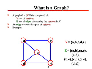
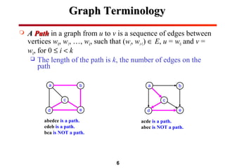
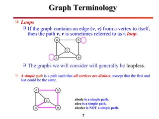
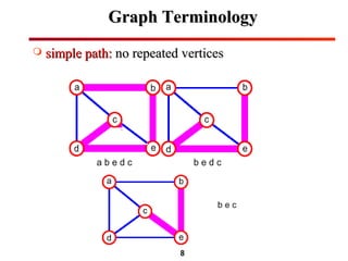
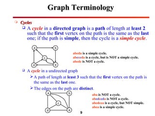
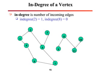
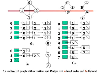
This document defines key graph terminology and concepts. It begins by defining what a graph is composed of - vertices and edges. It then discusses directed vs undirected graphs and defines common graph terms like adjacent vertices, paths, cycles, and more. The document also covers different ways to represent graphs, such as adjacency matrices and adjacency lists. Finally, it briefly introduces common graph search methods like breadth-first search and depth-first search.

![23
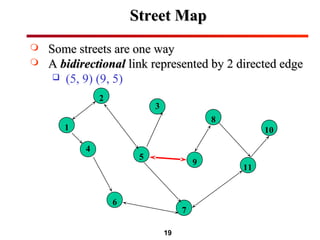
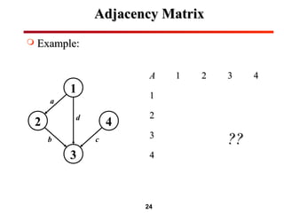
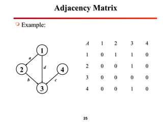
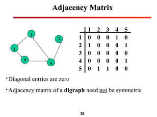
Adjacency MatrixAdjacency Matrix
AssumeAssume VV = {1, 2, …,= {1, 2, …, nn}}
AnAn adjacency matrixadjacency matrix represents the graph as arepresents the graph as a nn ×× nn
matrixmatrix AA::
A[i, j] = 1 if edge(i, j) ∈ E (or weight of edge)
= 0 if edge(i, j) ∉ E](https://image.slidesharecdn.com/graph-170105160416/85/Graph-23-320.jpg)
![31
Merits of Adjacency Matrix
From the adjacency matrix, to determine
the connection of vertices is easy
The degree of a vertex is
For a digraph (= directed graph), the row
sum is the out_degree, while the column
sum is the in_degree
adj mat i j
j
n
_ [ ][ ]
=
−
∑0
1
ind vi A j i
j
n
( ) [ , ]=
=
−
∑
0
1
outd vi A i j
j
n
( ) [ , ]=
=
−
∑
0
1](https://image.slidesharecdn.com/graph-170105160416/85/Graph-31-320.jpg)
![32
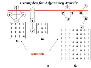
Adjacency ListAdjacency List
Adjacency list: for each vertexAdjacency list: for each vertex vv ∈∈ VV, store a list of vertices adjacent to, store a list of vertices adjacent to vv..
Adjacency list for vertexAdjacency list for vertex ii is a linear list of vertices adjacent from vertexis a linear list of vertices adjacent from vertex ii
Each adjacency list is a chain.Each adjacency list is a chain.
2
3
1
4
5
aList[1]
aList[5]
[2]
[3]
[4]
2 4
1 5
5
5 1
2 4 3
# of chain nodes = 2|E| (undirected graph)
# of chain nodes = |E| (digraph)](https://image.slidesharecdn.com/graph-170105160416/85/Graph-32-320.jpg)
![39
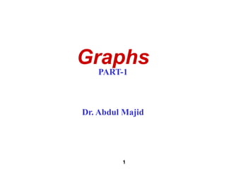
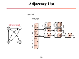
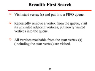
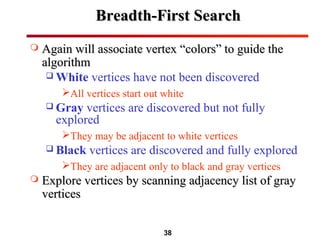
Breadth-First SearchBreadth-First Search
BFS(G, s) {BFS(G, s) {
// initialize vertices;// initialize vertices;
11 for each ufor each u ∈∈ V(G) – {s}{V(G) – {s}{
22 do color[u] = WHITEdo color[u] = WHITE
33 d[u] =d[u] = ∞∞ // distance from s to u// distance from s to u
44 p[u] = NILp[u] = NIL // predecessor or parent of u// predecessor or parent of u
}}
55 color[s] = GRAYcolor[s] = GRAY
66 d[s] = 0d[s] = 0
77 p[s] = NILp[s] = NIL
88 Q = Empty;Q = Empty;
99 Enqueue (Q,s);Enqueue (Q,s); // Q is a queue; initialize to s// Q is a queue; initialize to s
1010 while (Q not empty) {while (Q not empty) {
1111 u = Dequeue(Q);u = Dequeue(Q);
1212 for each vfor each v ∈∈ adj[u] {adj[u] {
1313 if (color[v] == WHITE)if (color[v] == WHITE)
1414 color[v] = GRAY;color[v] = GRAY;
1515 d[v] = d[u] + 1;d[v] = d[u] + 1;
1616 p[v] = u;p[v] = u;
1717 Enqueue(Q, v);Enqueue(Q, v);
}}
1818 color[u] = BLACK;color[u] = BLACK;
}}
}}
What does p[v] represent?
What does d[v] represent?](https://image.slidesharecdn.com/graph-170105160416/85/Graph-39-320.jpg)
![40
Breadth-First SearchBreadth-First Search
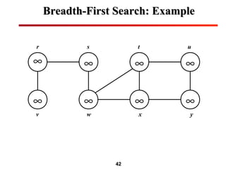
LinesLines 1-41-4 paint every vertex white, set d[u] to bepaint every vertex white, set d[u] to be
infinity for each vertex (u), and set p[u] the parentinfinity for each vertex (u), and set p[u] the parent
of every vertex to be NIL.of every vertex to be NIL.
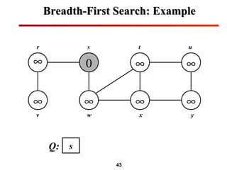
LineLine 55 paints the source vertex (s) gray.paints the source vertex (s) gray.
LineLine 66 initializes d[s] to 0.initializes d[s] to 0.
LineLine 77 sets the parent of the source to be NIL.sets the parent of the source to be NIL.
LinesLines 8-98-9 initialize Q to the queue containing justinitialize Q to the queue containing just
the vertex (s).the vertex (s).
TheThe whilewhile loop of linesloop of lines 10-1810-18 iterates as long asiterates as long as
there remain gray vertices, which are discoveredthere remain gray vertices, which are discovered
vertices that have not yet had their adjacency listsvertices that have not yet had their adjacency lists
fully examined.fully examined.
This while loop maintains the test in line 10, the
queue Q consists of the set of the gray vertices.](https://image.slidesharecdn.com/graph-170105160416/85/Graph-40-320.jpg)
![41
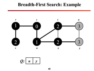
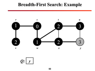
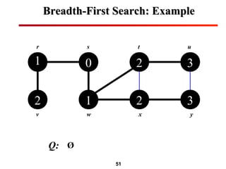
Breadth-First SearchBreadth-First Search
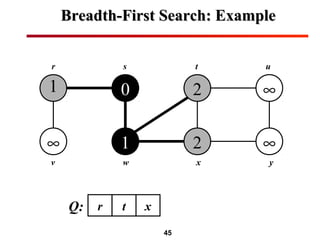
Prior to the first iteration in linePrior to the first iteration in line 1010, the only gray vertex, and, the only gray vertex, and
the only vertex in Q, is the source vertex (s).the only vertex in Q, is the source vertex (s).
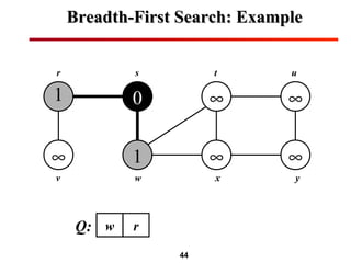
LineLine 1111 determines the gray vertex (u) at the head of the queuedetermines the gray vertex (u) at the head of the queue
Q and removes it from Q.Q and removes it from Q.
TheThe forfor loop of linesloop of lines 12-1712-17 considers each vertex (v) in theconsiders each vertex (v) in the
adjacency list of (u).adjacency list of (u).
If (v) is white, then it has not yet been discovered, and theIf (v) is white, then it has not yet been discovered, and the
algorithm discovers it by executing linesalgorithm discovers it by executing lines 14-1714-17..
It is first grayed, and its distance d[v] is set to d[u]+1.
Then, u is recorded as its parent.
Finally, it is placed at the tail of the queue Q.
When all the vertices on (u’s) adjacency list have beenWhen all the vertices on (u’s) adjacency list have been
examined, u is blackened in lineexamined, u is blackened in line 1818..](https://image.slidesharecdn.com/graph-170105160416/85/Graph-41-320.jpg)
![52
BFS: The Code AgainBFS: The Code Again
BFS(G, s) {BFS(G, s) {
// initialize vertices// initialize vertices
for each ufor each u ∈∈ V(G) – {s}{V(G) – {s}{
do color[u] = WHITEdo color[u] = WHITE
d[u] =d[u] = ∞∞
p[u] = NILp[u] = NIL
}}
color[s] = GRAY;color[s] = GRAY;
d[s] = 0;d[s] = 0;
p[s] = NIL;p[s] = NIL;
Q = Empty;Q = Empty;
Enqueue (Q,s);Enqueue (Q,s);
while (Q not empty) {while (Q not empty) {
u = Dequeue(Q);u = Dequeue(Q);
for each vfor each v ∈∈ adj[u] {adj[u] {
if (color[v] == WHITE)if (color[v] == WHITE)
color[v] = GRAY;color[v] = GRAY;
d[v] = d[u] + 1;d[v] = d[u] + 1;
p[v] = u;p[v] = u;
Enqueue(Q, v);Enqueue(Q, v);
}}
color[u] = BLACK;color[u] = BLACK;
}}
}}
What will be the running time?
Touch every vertex: O(V)
u = every vertex, but only once
So v = every vertex
that appears in
some other vert’s
adjacency list Total running time: O(V+E)
O(E)](https://image.slidesharecdn.com/graph-170105160416/85/Graph-52-320.jpg)