Downloaded 173 times
![References
36
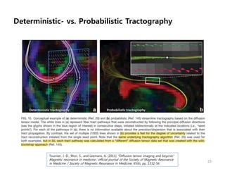
[1] Tournier, J.-D., Mori, S., and Leemans, A. (2011).
“Diffusion tensor imaging and beyond.” Magnetic
resonance in medicine : official journal of the Society
of Magnetic Resonance in Medicine / Society of
Magnetic Resonance in Medicine, 65(6), pp. 1532-56.
[2] Callaghan, P., Codd, S., and Seymour, J. (1999).
“Spatial coherence phenomena arising from
translational spin motion in gradient spin echo
experiments.” Concepts in Magnetic Resonance, 11(4),
pp. 181–202.
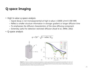
[3] Cohen, Y. and Assaf, Y. (2002). “High b-value q-
space analyzed diffusion-weighted MRS and MRI in
neuronal tissues - a technical review.” NMR in
biomedicine, 15(7-8), pp. 516-42.](https://image.slidesharecdn.com/2011-10-04diffusiontensorimaging-140520023516-phpapp01/85/Diffusion-Tensor-Imaging-2011-10-04-36-320.jpg)

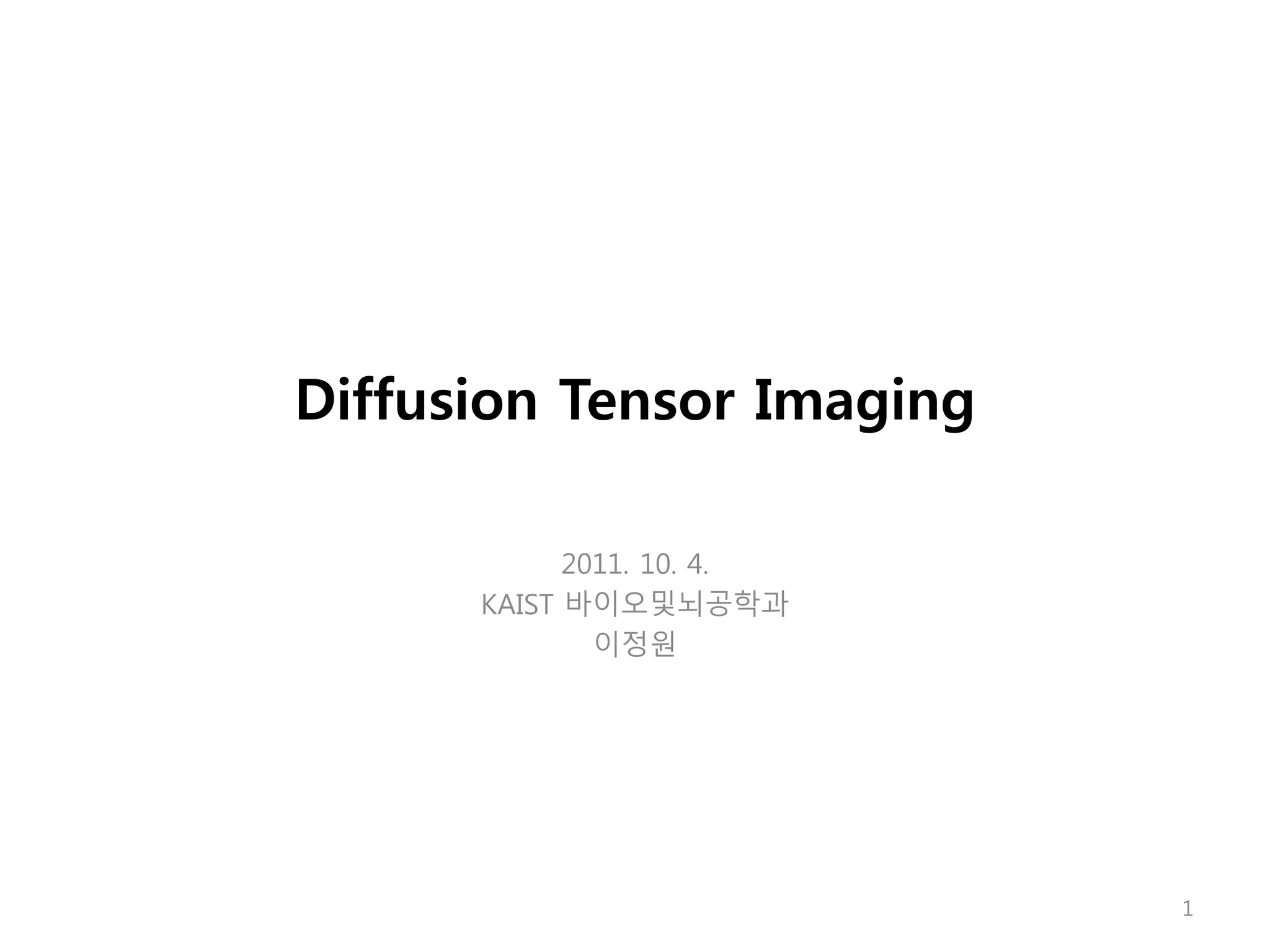
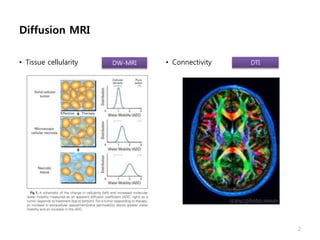
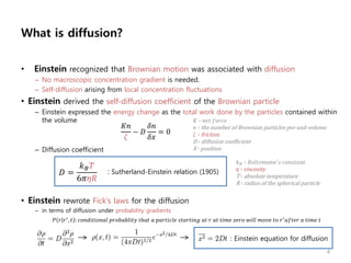
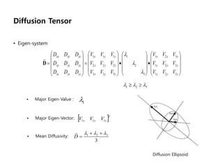
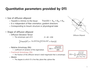
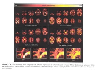
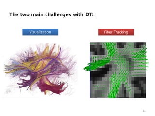
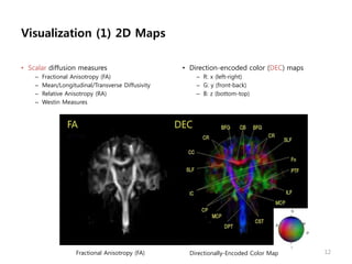
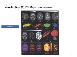
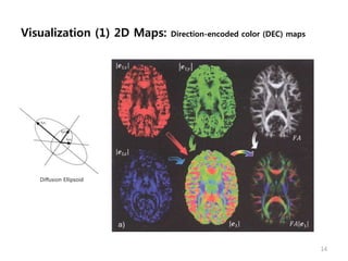
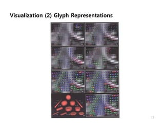
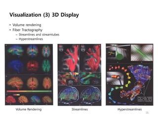
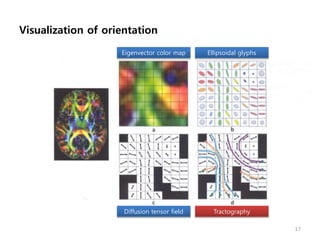
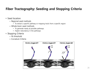
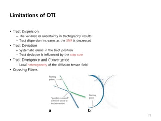
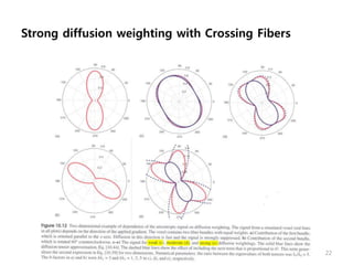
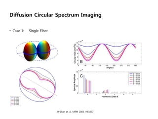
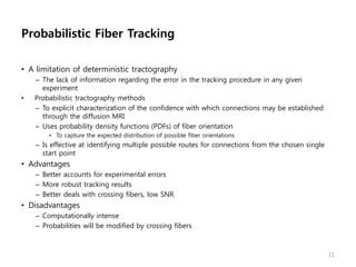
This document provides an overview of diffusion tensor imaging (DTI). It describes how DTI can be used to measure the diffusion of water molecules in tissue to determine tissue cellularity and connectivity. Key aspects covered include diffusion anisotropy, the diffusion tensor, quantitative DTI parameters like fractional anisotropy, visualization techniques like fiber tractography, limitations of DTI like issues with crossing fibers, and more advanced methods like probabilistic fiber tracking and high b-value q-space imaging.


![CASE_PRESENTATION_ON_subdural_hematoma(SDH)[1 FINAL PPT]-1.pptx](https://cdn.slidesharecdn.com/ss_thumbnails/casepresentationonsubduralhematomasdh1finalppt-1-260129172522-d405d375-thumbnail.jpg?width=640&height=640&fit=bounds)


