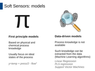
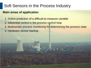
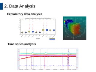
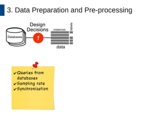
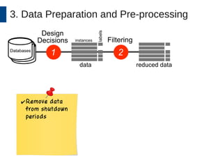
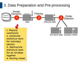
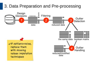
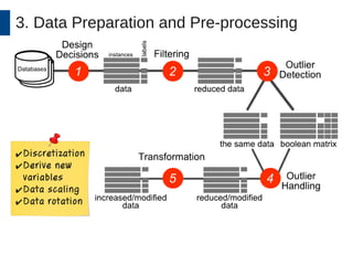
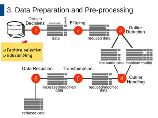
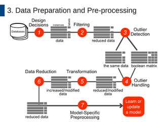
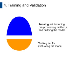
From sensor readings to prediction: on the 
process of developing practical soft sensors 
Marcin Budka1, Mark Eastwood2, Bogdan Gabrys1, Petr Kadlec3, Manuel Martin Salvador1, 
Stephanie Schwan3, Athanasios Tsakonas1, Indre Zliobaite4 
1Bournemouth University, UK 
2Coventry University, UK 
3Evonik Industries, Germany 
4Aalto University and HIIT, Finland IDA 2014. Leuven, Belgium
Outline 
1. INFER project 
2. Sensors, sensors, sensors 
3. Easy vs difficult 
4. Soft Sensors 
4.1. Soft Sensors: models 
4.2. Soft Sensors in the Process Industry 
4.3. An unsuccessful soft sensor 
4.4. A successful soft sensor 
4.5. How to build a successful data-driven soft sensor? 
4.5.1. Performance goal and evaluation criteria 
4.5.2. Data Analysis 
4.5.3. Data Preparation and Pre-processing 
4.5.4. Training and validation 
5. Our case study 
5.1. Versions of the data 
5.2. Evaluation 
6. Conclusion
Sensors, sensors, sensors
Sensors, sensors, sensors 
SSEENNSSOORRSS 
Image copyright by Disney Pixar. Qualifies fair usage. 
SSEENNSSOORRSS EEVVEERRYYWWHHEERREE
Easy vs difficult 
Easy-to-measure variables Difficult-to-measure variables 
Temperature 
Polymerisation progress 
Pressure 
Humidity 
Flow 
Fermentation progress 
Concentration
Soft Sensors 
Soft sensors are computational models 
that aggregate readings of physical sensors 
Soft sensors operate online using streams of sensor readings, 
therefore they need to be robust to noise 
and adaptive to changes over time.
Soft Sensors: models 
First principle models Data-driven models 
Based on physical and 
chemical process 
knowledge 
Usually focus on ideal 
states of the process 
Process knowledge is not 
available 
Such knowledge can be 
extracted from the data 
(Machine Learning algorithms) 
y=temp + press/2 - flow2 
Linear Regression 
PLS regression 
Support Vector Machines 
π
Soft Sensors in the Process Industry 
Main areas of application 
1. Online prediction of a difficult-to-measure variable 
2. Inferential control in the process control loop 
3. Multivariate process monitoring for determining the process state 
4. Hardware sensor backup
An unsuccessful soft sensor 
Image copyright by Disney Pixar. Qualifies fair usage.
A successful soft sensor 
Implemented into the process online environment 
Accepted by the process operators 
Requirements: 
• Reasonable performance 
• Stable 
• Predictable 
• Transparency 
• Automation 
• Robustness 
• Adaptivity
A successful soft sensor 
Image copyright by Disney Pixar. Qualifies fair usage.
How to build a successful 
data-driven soft sensor? 
Proposed framework: 
1) Setting up the performance goals and evaluation criteria 
2) Data analysis (exploratory) 
3) Data preparation and preprocessing 
4) Training and validating the predictive model 
Keep domain expert in the loop from the beginning
1. Performance goals and evaluation criteria 
Performance goal examples: 
● Classification accuracy > 85% 
● Processing time per sample < 1s 
Evaluation criteria: 
● Qualitative evaluation: 
● Transparency 
● Model complexity 
● Quantitative evaluation: 
● RMSE 
● MAE 
● Jitter 
● Confidence
2. Data Analysis 
Exploratory data analysis 
Time series analysis
3. Data Preparation and Pre-processing 
✔Queries from 
databases 
✔Sampling rate 
✔Synchronization
3. Data Preparation and Pre-processing 
✔Remove data 
from shutdown 
periods
3. Data Preparation and Pre-processing 
1. Physical 
constraints 
2. Univariate 
statistical tests 
for individual 
sensors 
3. Multivariate 
statistical tests 
for all variables 
together 
4. Missing values
3. Data Preparation and Pre-processing 
✔If outliers=noise, 
replace them 
with missing 
values imputation 
techniques
3. Data Preparation and Pre-processing 
✔Discretization 
✔Derive new 
variables 
✔Data scaling 
✔Data rotation
3. Data Preparation and Pre-processing 
✔Feature selection 
✔Subsampling
3. Data Preparation and Pre-processing
4. Training and Validation 
Training set for tuning 
pre-processing methods 
and building the model 
Testing set for 
evaluating the model
Our case study 
Background picture is Creative Commons by Paul Joyce 
Real industrial dataset from a debutanizer column 
3 years of operation 
189,193 records (every 5 min) 
85 sensors 
Target: concentration of the product
Versions of the data 
Code Description 
RAW no pre-processing (188752 training / 21859 testing) 
SUB subsampling (every 1h – 15611 training / 1822 testing) 
SYN features are synchronised 
FET-E 20 features selected using the first 1000 training samples 
FET-L 20 features selected using the latest 1000 training samples 
FRA additional features derived by computing the fractal dimension 
DIF original values are replaced with the first derivative with respect 
to time
Evaluation 
Partial Least Squares regression → transparency 
MAE = Mean Absolute Error 
Data #1 MAE #1 Data #2 MAE #2 % improvement 
RAW 225 RAW-SYN 222 1% 
SUB 227 SUB-SYN 221 3% 
RAW-FET-E 228 RAW-FET-L 198 13% 
RAW-SYN-FET-E 245 RAW-SYN-FET-L 201 18% 
SUB-FET-E 236 SUB-FET-L 193 18% 
SUB-SYN-FET-E 215 SUB-SYN-FET-L 185 14% 
SUB-DIF 41.8 SUB-DIF-SYN 35.3 16% 
SUB-DIF 41.8 SUB-DIF-FRA 32.4 22%
Evaluation (cont.) 
● Feature synchronization can have positive or negative effect 
in prediction 
● Adaptive feature selection using the latest samples is 
beneficial → Feature importance change over time 
● Taking into account temporal differences is very beneficial 
→ Product concentration does not change suddenly
Conclusion 
✔Framework for building a successful soft sensor 
✔Case study with real data from industrial production process 
✔Adaptive pre-processing could be very beneficial (and 
sometimes a must) 
Future directions: 
Extend feature space with autoregressive features 
Filter out the effects of data compression 
Ongoing work: 
Automation and adaptation of data stream pre-processing
Thanks! 
Slides available in http://slideshare.net/draxus 
msalvador@bournemouth.ac.uk

From sensor readings to prediction: on the process of developing practical soft sensors

  • 1.
    From sensor readingsto prediction: on the process of developing practical soft sensors Marcin Budka1, Mark Eastwood2, Bogdan Gabrys1, Petr Kadlec3, Manuel Martin Salvador1, Stephanie Schwan3, Athanasios Tsakonas1, Indre Zliobaite4 1Bournemouth University, UK 2Coventry University, UK 3Evonik Industries, Germany 4Aalto University and HIIT, Finland IDA 2014. Leuven, Belgium
  • 2.
    Outline 1. INFERproject 2. Sensors, sensors, sensors 3. Easy vs difficult 4. Soft Sensors 4.1. Soft Sensors: models 4.2. Soft Sensors in the Process Industry 4.3. An unsuccessful soft sensor 4.4. A successful soft sensor 4.5. How to build a successful data-driven soft sensor? 4.5.1. Performance goal and evaluation criteria 4.5.2. Data Analysis 4.5.3. Data Preparation and Pre-processing 4.5.4. Training and validation 5. Our case study 5.1. Versions of the data 5.2. Evaluation 6. Conclusion
  • 4.
  • 5.
    Sensors, sensors, sensors SSEENNSSOORRSS Image copyright by Disney Pixar. Qualifies fair usage. SSEENNSSOORRSS EEVVEERRYYWWHHEERREE
  • 6.
    Easy vs difficult Easy-to-measure variables Difficult-to-measure variables Temperature Polymerisation progress Pressure Humidity Flow Fermentation progress Concentration
  • 7.
    Soft Sensors Softsensors are computational models that aggregate readings of physical sensors Soft sensors operate online using streams of sensor readings, therefore they need to be robust to noise and adaptive to changes over time.
  • 8.
    Soft Sensors: models First principle models Data-driven models Based on physical and chemical process knowledge Usually focus on ideal states of the process Process knowledge is not available Such knowledge can be extracted from the data (Machine Learning algorithms) y=temp + press/2 - flow2 Linear Regression PLS regression Support Vector Machines π
  • 9.
    Soft Sensors inthe Process Industry Main areas of application 1. Online prediction of a difficult-to-measure variable 2. Inferential control in the process control loop 3. Multivariate process monitoring for determining the process state 4. Hardware sensor backup
  • 10.
    An unsuccessful softsensor Image copyright by Disney Pixar. Qualifies fair usage.
  • 11.
    A successful softsensor Implemented into the process online environment Accepted by the process operators Requirements: • Reasonable performance • Stable • Predictable • Transparency • Automation • Robustness • Adaptivity
  • 12.
    A successful softsensor Image copyright by Disney Pixar. Qualifies fair usage.
  • 13.
    How to builda successful data-driven soft sensor? Proposed framework: 1) Setting up the performance goals and evaluation criteria 2) Data analysis (exploratory) 3) Data preparation and preprocessing 4) Training and validating the predictive model Keep domain expert in the loop from the beginning
  • 14.
    1. Performance goalsand evaluation criteria Performance goal examples: ● Classification accuracy > 85% ● Processing time per sample < 1s Evaluation criteria: ● Qualitative evaluation: ● Transparency ● Model complexity ● Quantitative evaluation: ● RMSE ● MAE ● Jitter ● Confidence
  • 15.
    2. Data Analysis Exploratory data analysis Time series analysis
  • 16.
    3. Data Preparationand Pre-processing ✔Queries from databases ✔Sampling rate ✔Synchronization
  • 17.
    3. Data Preparationand Pre-processing ✔Remove data from shutdown periods
  • 18.
    3. Data Preparationand Pre-processing 1. Physical constraints 2. Univariate statistical tests for individual sensors 3. Multivariate statistical tests for all variables together 4. Missing values
  • 19.
    3. Data Preparationand Pre-processing ✔If outliers=noise, replace them with missing values imputation techniques
  • 20.
    3. Data Preparationand Pre-processing ✔Discretization ✔Derive new variables ✔Data scaling ✔Data rotation
  • 21.
    3. Data Preparationand Pre-processing ✔Feature selection ✔Subsampling
  • 22.
    3. Data Preparationand Pre-processing
  • 23.
    4. Training andValidation Training set for tuning pre-processing methods and building the model Testing set for evaluating the model
  • 24.
    Our case study Background picture is Creative Commons by Paul Joyce Real industrial dataset from a debutanizer column 3 years of operation 189,193 records (every 5 min) 85 sensors Target: concentration of the product
  • 25.
    Versions of thedata Code Description RAW no pre-processing (188752 training / 21859 testing) SUB subsampling (every 1h – 15611 training / 1822 testing) SYN features are synchronised FET-E 20 features selected using the first 1000 training samples FET-L 20 features selected using the latest 1000 training samples FRA additional features derived by computing the fractal dimension DIF original values are replaced with the first derivative with respect to time
  • 26.
    Evaluation Partial LeastSquares regression → transparency MAE = Mean Absolute Error Data #1 MAE #1 Data #2 MAE #2 % improvement RAW 225 RAW-SYN 222 1% SUB 227 SUB-SYN 221 3% RAW-FET-E 228 RAW-FET-L 198 13% RAW-SYN-FET-E 245 RAW-SYN-FET-L 201 18% SUB-FET-E 236 SUB-FET-L 193 18% SUB-SYN-FET-E 215 SUB-SYN-FET-L 185 14% SUB-DIF 41.8 SUB-DIF-SYN 35.3 16% SUB-DIF 41.8 SUB-DIF-FRA 32.4 22%
  • 27.
    Evaluation (cont.) ●Feature synchronization can have positive or negative effect in prediction ● Adaptive feature selection using the latest samples is beneficial → Feature importance change over time ● Taking into account temporal differences is very beneficial → Product concentration does not change suddenly
  • 28.
    Conclusion ✔Framework forbuilding a successful soft sensor ✔Case study with real data from industrial production process ✔Adaptive pre-processing could be very beneficial (and sometimes a must) Future directions: Extend feature space with autoregressive features Filter out the effects of data compression Ongoing work: Automation and adaptation of data stream pre-processing
  • 29.
    Thanks! Slides availablein http://slideshare.net/draxus msalvador@bournemouth.ac.uk