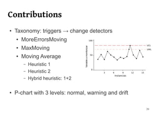
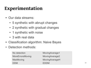
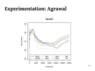
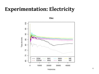
The document summarizes Manuel Martín Salvador's master's thesis on handling concept drift in data streams. It discusses concept drift, online learning approaches, evaluation methods, and taxonomy of concept drift handling methods. The contributions include developing new change detection heuristics called MoreErrorsMoving, MaxMoving, and Moving Average (with two variants), as well as a hybrid approach combining the heuristics.

1. Handling concept drift in data
stream mining
Student: Manuel Martín Salvador
Supervisors: Luis M. de Campos and Silvia Acid
Master in Soft Computing and Intelligent Systems
Department of Computer Science and Artificial Intelligence
University of Granada

2. Who am I?
1. Current: PhD Student in Bournemouth University
2. Previous:
● Computer Engineering in University of Granada
(2004-2009)
● Programmer and SCRUM Master in Fundación
I+D del Software Libre (2009-2010)
● Master in Soft Computing and Intelligent
Systems in University of Granada (2010-2011)
● Researcher in Department of Computer Science
and Artificial Intelligence of UGR (2010-2012)

3. Index
1. Data streams
2. Online Learning
3. Evaluation
4. Taxonomy of methods
5. Contributions
6. MOA
7. Experimentation
8. Conclusions and future work
3

4. Data streams
1. Continous flow of instances.
● In classification: instance = (a1 , a2 , …, an , c)
2. Unlimited size
3. May have changes in the underlying distribution of the
data → concept drift
4
Image: I. Žliobaitė thesis

5. Concept drifts
● It happens when the data from a stream changes its
probability distribution ПS1 to another ПS2. Potential
causes:
● Change in P(C)
● Change in P(X|C)
● Change in P(C|X)
● Unpredictable
● For example: spam
5

6. Gradual concept drift
6
Image: I. Žliobaitė thesis

7. Types of concept drifts
7
Image: D. Brzeziński thesis

8. Types of concept drifts
8
Image: D. Brzeziński thesis

9. Example: STAGGER
color=red color=green size=medium
Class=true if → and or or
size=small shape=cricle size=large
9
Image: Kolter & Maloof

10. Online learning (incremental)
● Goal: incrementally learn a classifier at least as
accurate as if it had been trained in batch
● Requirements:
1. Incremental
2. Single pass
3. Limited time and memory
4. Any-time learning: availability of the model
10

11. Online learning (incremental)
● Goal: incrementally learn a classifier at least as
accurate as if it had been trained in batch
● Requirements:
1. Incremental
2. Single pass
3. Limited time and memory
4. Any-time learning: availability of the model
● Nice to have: deal with concept drift.
11

12. Evaluation
Several criteria:
● Time → seconds
● Memory → RAM/hour
● Generalizability of the model → % success
● Detecting concept drift → detected drifts, false
positives and false negatives
12

13. Evaluation
Several criteria:
● Time → seconds
● Memory → RAM/hour
● Generalizability of the model → % success
● Detecting concept drift → detected drifts, false
positives and false negatives
Problem: we can't use the traditional techniques for
evaluation (i.e. cross validation). → Solution: new
strategies.
13

14. Evaluation: prequential
● Test y training each instance. errors
processed instances
● Is a pessimistic estimator: holds the errors since the
beginning of the stream. → Solution: forgetting
mechanisms (sliding window and fading factor).
errors inside window
Sliding window: window size …...
currentError⋅errors
Fading factor: 1⋅processed instances …...
Advantages: All instances are used for training.
Useful for data streams with concept drifts. 14

15. Evaluation: comparing
Which method is better? 15

16. Evaluation: comparing
Which method is better? → AUC 16

17. Evaluation: drift detection
● First detected: correct.
● Following detected: false positives.
● Not detected: false negatives.
● Distance = correct – real.
17

18. Taxonomy of methods
● Change detectors
Learners with ● Training windows
triggers ● Adaptive sampling
✔ Advantages: can be used by any classification algorithm.
✗ Disadvantages: usually, once detected a change, they discard the old
model and relearn a new one.
18

19. Taxonomy of methods
● Change detectors
Learners with ● Training windows
triggers ● Adaptive sampling
✔ Advantages: can be used by any classification algorithm.
✗ Disadvantages: usually, once detected a change, they discard the old
model and relearn a new one.
● Adaptive ensembles
Evolving ● Instance weighting
Learners ● Feature space
● Base model specific
✔ Advantages: they continually adapt the model over time
✗ Disadvantages: they don't detect changes. 19

20. Contributions
● Taxonomy: triggers → change detectors
● MoreErrorsMoving
● MaxMoving
● Moving Average
– Heuristic 1
– Heuristic 2
– Hybrid heuristic: 1+2
● P-chart with 3 levels: normal, warning and drift
20

21. Contributions: MoreErrorsMoving
● n latest results of classification are monitored →
History = {ei , ei+1 , …, ei+n} (i.e. 0,0,1,1)
● History error rate:
● The consecutive declines are controlled
● At each time step:
● If ci - 1 < ci (more errors) → declines++
● If ci - 1 > ci (less errors) → declines=0
● If ci - 1 = ci (same) → declines don't change
21

22. Contributions: MoreErrorsMoving
● If consecutive declines > k → enable Warning
● If consecutive declines > k+d → enable Drift
● Otherwise → enable Normality
22

23. Contributions: MoreErrorsMoving
History = 8
Warning = 2
Drift = 4
Detected
drifts:
46 y 88
Distance to real drifts:
46-40 = 6
88-80 = 8
23

24. Contributions: MaxMoving
● n latest success accumulated rates are monitored since
the last change
● History={ai , ai+1 , …, ai+n} (i.e. H={2/5, 3/6, 4/7, 4/8})
● History maximum:
● The consecutive declines are controlled
● At each time step:
● If mi < mi - 1 → declines++
● If mi > mi - 1 → declines=0
● If mi = mi - 1 → declines don't change
24

25. Contributions: MaxMoving
History = 4
Warning = 4
Drift = 8
Detected
drifts:
52 y 90
Distance to real drifts:
52-40 = 12
90-80 = 10
25

26. Contributions: Moving Average
Goal: to smooth accuracy rates for better detection.
26

27. Contributions: Moving Average 1
● m latest success accumulated rates are smoothed → Simple
moving average (unweighted mean)
● The consecutive declines are controlled
● At each time step:
● If st < st - 1 → declines++
● If st > st - 1 → declines = 0
● If st = st - 1 → declines don't change
27

28. Contributions: Moving Average 1
Smooth = 32
Warning = 4
Drift = 8
Detected
drifts:
49 y 91
Distance to real drifts:
49-40 = 9
91-80 = 11
28

29. Contributions: Moving Average 2
● History of size n with the smoothed success rates →
History={si, si+1, …, si+n}
● History maximum:
● Difference between st and mt – 1 is monitored
● At each time step:
● If mt – 1 - st > u → enable Warning
● If mt – 1 - st > v → enable Drift
● Otherwise → enable Normality
● Suitable for abrupt changes
29

30. Contributions: Moving Average 2
Smooth = 4
History = 32
Warning = 2%
Drift = 4%
Detected
drifts:
44 y 87
Distance to real drifts:
44-40 = 4
87-80 = 7
30

31. Contributions: Moving Average Hybrid
● Heuristics 1 and 2 are combined:
● If Warning1 or Warning2 → enable Warning
● If Drift1 or Drift2 → enable Drift
● Otherwise → enable Normality
31

32. MOA: Massive Online Analysis
● Framework for data stream mining. Algorithms for
classification, regression and clustering.
● University of Waikato → WEKA integration.
● Graphical user interface and command line.
● Data stream generators.
● Evaluation methods (holdout and prequential).
● Open source and free.
http://moa.cs.waikato.ac.nz
32

33. Experimentation
● Our data streams:
● 5 synthetic with abrupt changes
● 2 synthetic with gradual changes
● 1 synthetic with noise
● 3 with real data
33

34. Experimentation
● Our data streams:
● 5 synthetic with abrupt changes
● 2 synthetic with gradual changes
● 1 synthetic with noise
● 3 with real data
● Classification algorithm: Naive Bayes
34

35. Experimentation
● Our data streams:
● 5 synthetic with abrupt changes
● 2 synthetic with gradual changes
● 1 synthetic with noise
● 3 with real data
● Classification algorithm: Naive Bayes
● Detection methods:
No detection MovingAverage1
MoreErrorsMoving MovingAverage2
MaxMoving MovingAverageH
DDM EDDM 35

36. Experimentation
● Parameters tuning:
● 4 streams y 5 methods → 288 experiments
36

37. Experimentation
● Parameters tuning:
● 4 streams y 5 methods → 288 experiments
● Comparative study:
● 11 streams y 8+1 methods → 99 experiments
37

38. Experimentation
● Parameters tuning:
● 4 streams y 5 methods → 288 experiments
● Comparative study:
● 11 streams y 8+1 methods → 99 experiments
● Evaluation: prequential
38

39. Experimentation
● Parameters tuning:
● 4 streams y 5 methods → 288 experiments
● Comparative study:
● 11 streams y 8+1 methods → 99 experiments
● Evaluation: prequential
● Measurements:
● AUC: area under the curve of accumulated success
rates
● Number of correct drifts
● Distance to drifts
● False positives and false negatives 39

40. Experimentation: Agrawal
40

41. Experimentation: Electricity
41

42. Conclussions of experimentation
1. With abrupt changes:
● More victories: DDM and MovingAverageH
● Best in mean: MoreErrorsMoving → very responsive
2. With gradual changes:
● Best: DDM and EDDM
● Problem: many false positives → parameter tunning only with abrupt
changes
3. With noise:
● Only winner: DDM
● Problem: noise sensitive → parameter tunning only with no-noise data
4. Real data:
● Best: MovingAverage1 and MovingAverageH
42

43. Conclussions of this work
1. Our methods are competitive, although sensitive to
the parameters → Dynamic fit
2. Evaluation is not trivial → Standardization is needed
3. Large field of application in industry
4. Hot topic: last papers from 2011 + conferences
43

44. Future work
1. Dynamic adjustment of parameters.
2. Measuring the abruptness of change for:
● Using differents forgetting mechanisms.
● Setting the degree of change of the model.
3. Develop an incremental learning algorithm which
allows partial changes of the model when a drift is
detected.
44

45. Thank you
45