Calculus course presentation

1. Calculus
For Computer Science @ BUKC

2. Topics for Week 5 (Lecture 1)
•Derivative; Rules – How to find derivative of various
(types of) functions

3. Derivatives of Polynomials
and Exponential Functions

4. Derivatives of Polynomials and Exponential Functions
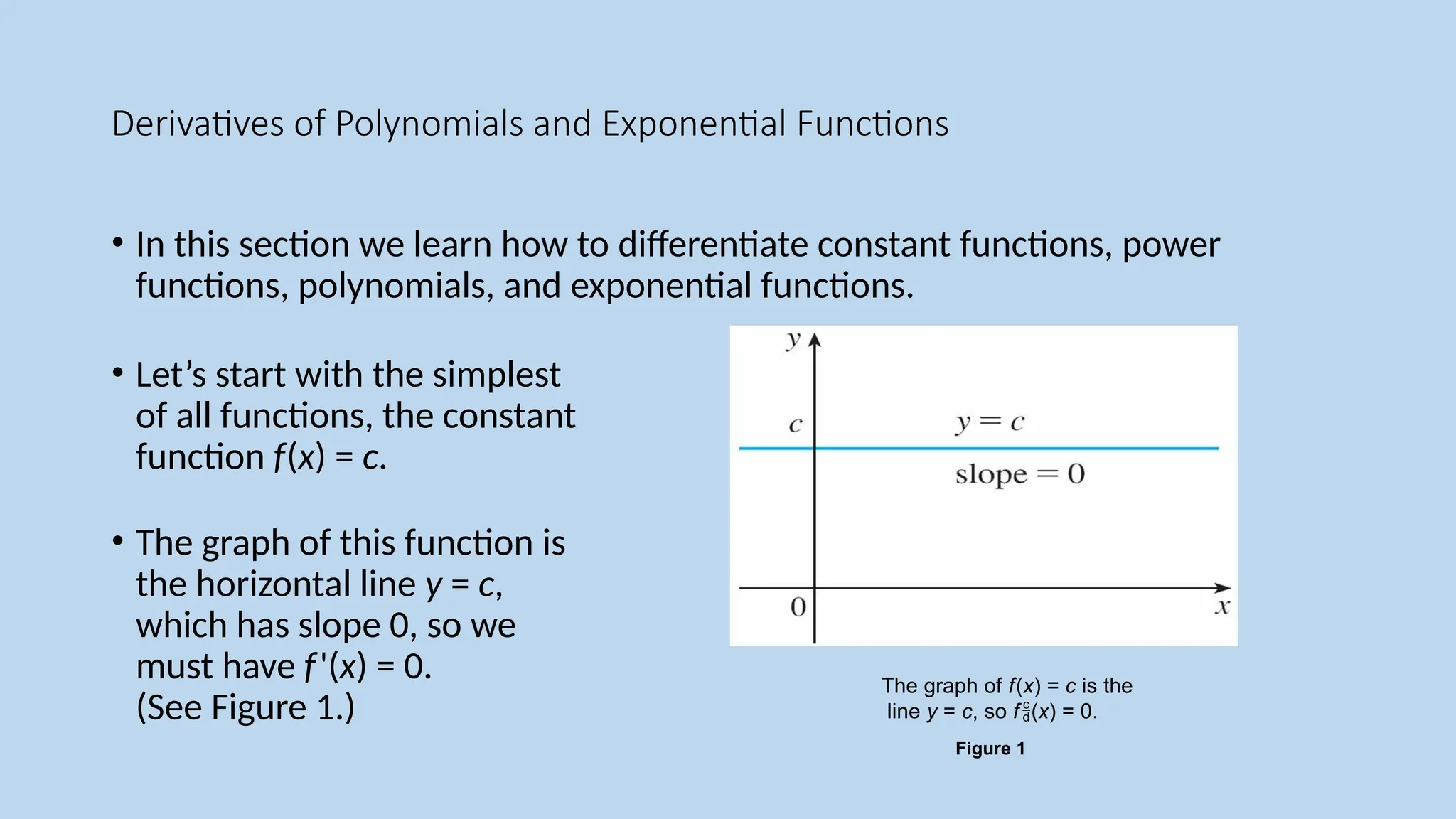
• In this section we learn how to differentiate constant functions, power
functions, polynomials, and exponential functions.
• Let’s start with the simplest
of all functions, the constant
function f(x) = c.
• The graph of this function is
the horizontal line y = c,
which has slope 0, so we
must have f'(x) = 0.
(See Figure 1.)
Figure 1
The graph of f(x) = c is the
line y = c, so f(x) = 0.

5. Derivatives of Polynomials and Exponential Functions
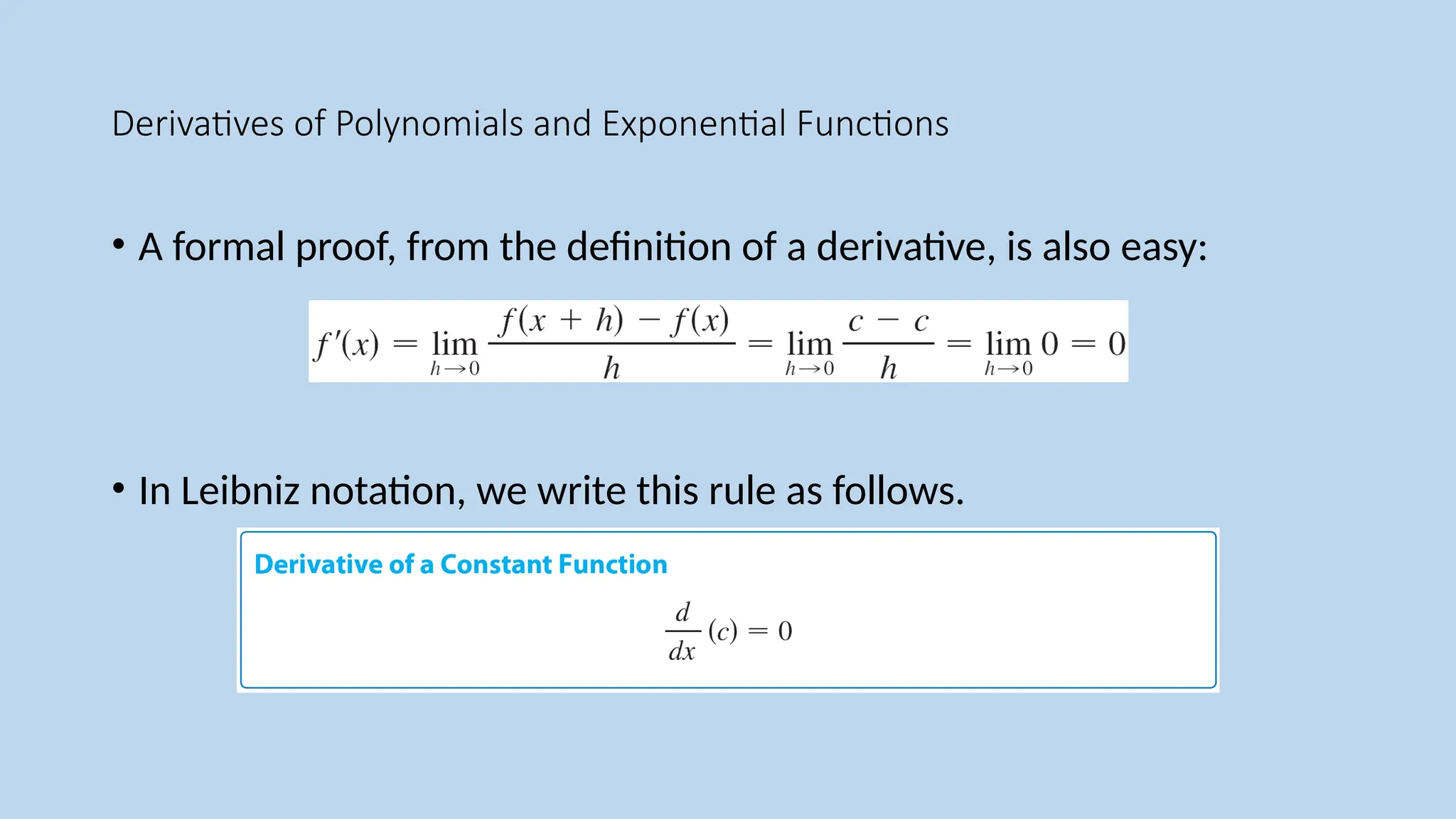
• A formal proof, from the definition of a derivative, is also easy:
• In Leibniz notation, we write this rule as follows.

6. Power Functions

7. Power Functions
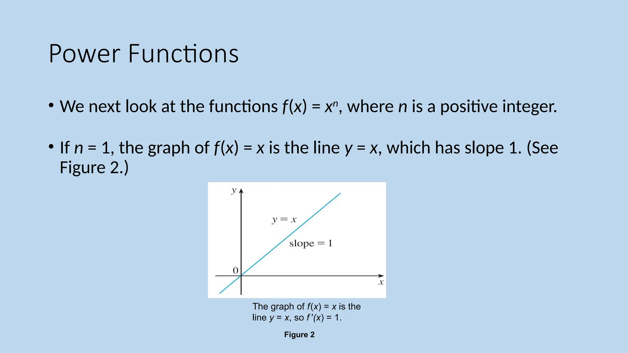
• We next look at the functions f(x) = xn
, where n is a positive integer.
• If n = 1, the graph of f(x) = x is the line y = x, which has slope 1. (See
Figure 2.)
Figure 2
The graph of f(x) = x is the
line y = x, so f '(x) = 1.

8. Power Functions
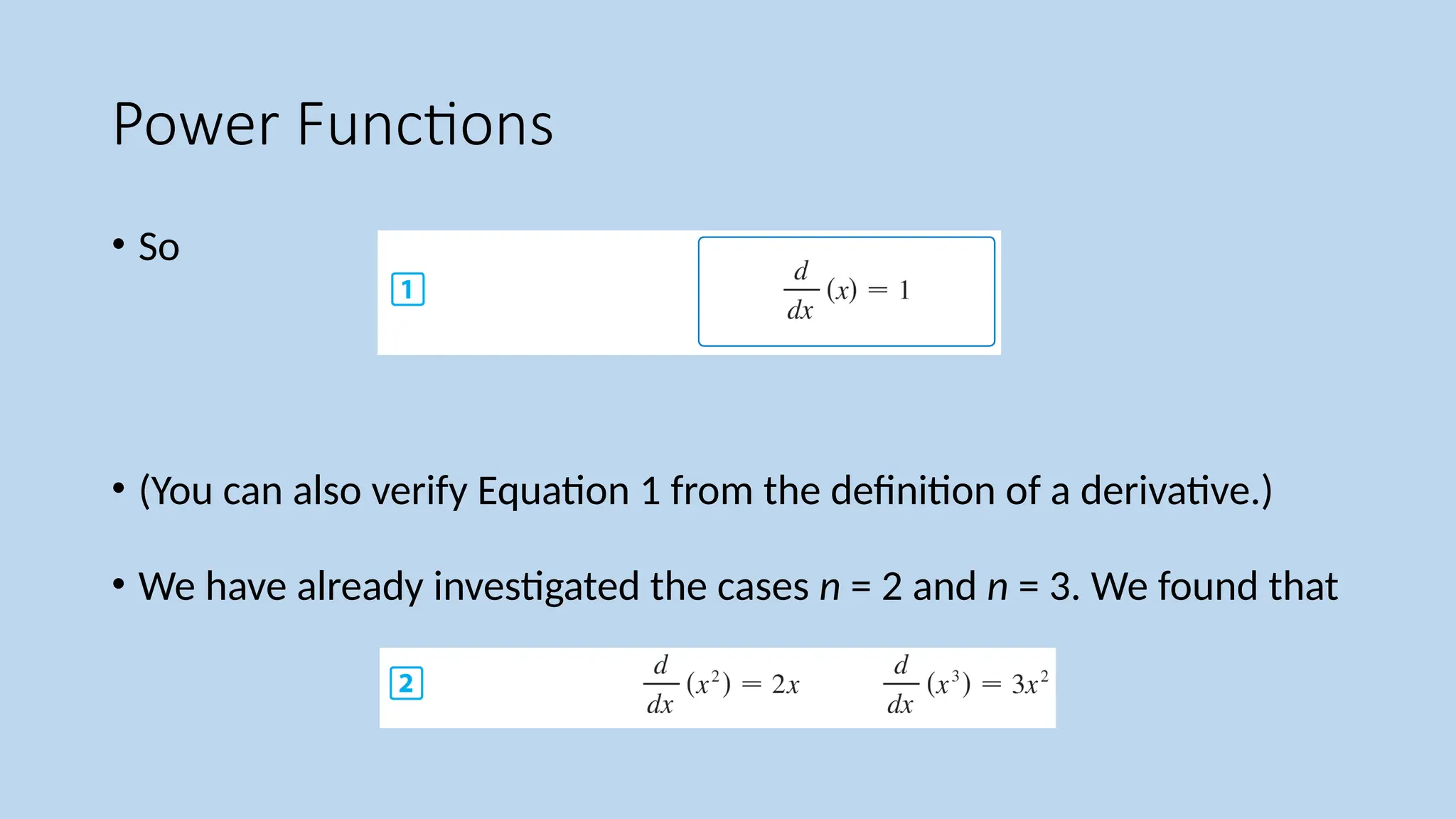
• So
• (You can also verify Equation 1 from the definition of a derivative.)
• We have already investigated the cases n = 2 and n = 3. We found that

9. Power Functions
For n = 4 we find the derivative of f(x) = x4
as follows:

10. Power Functions
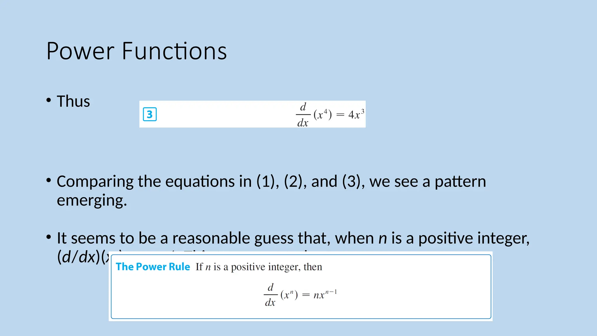
• Thus
• Comparing the equations in (1), (2), and (3), we see a pattern
emerging.
• It seems to be a reasonable guess that, when n is a positive integer,
(d/dx)(xn
) = nxn –1
. This turns out to be true.

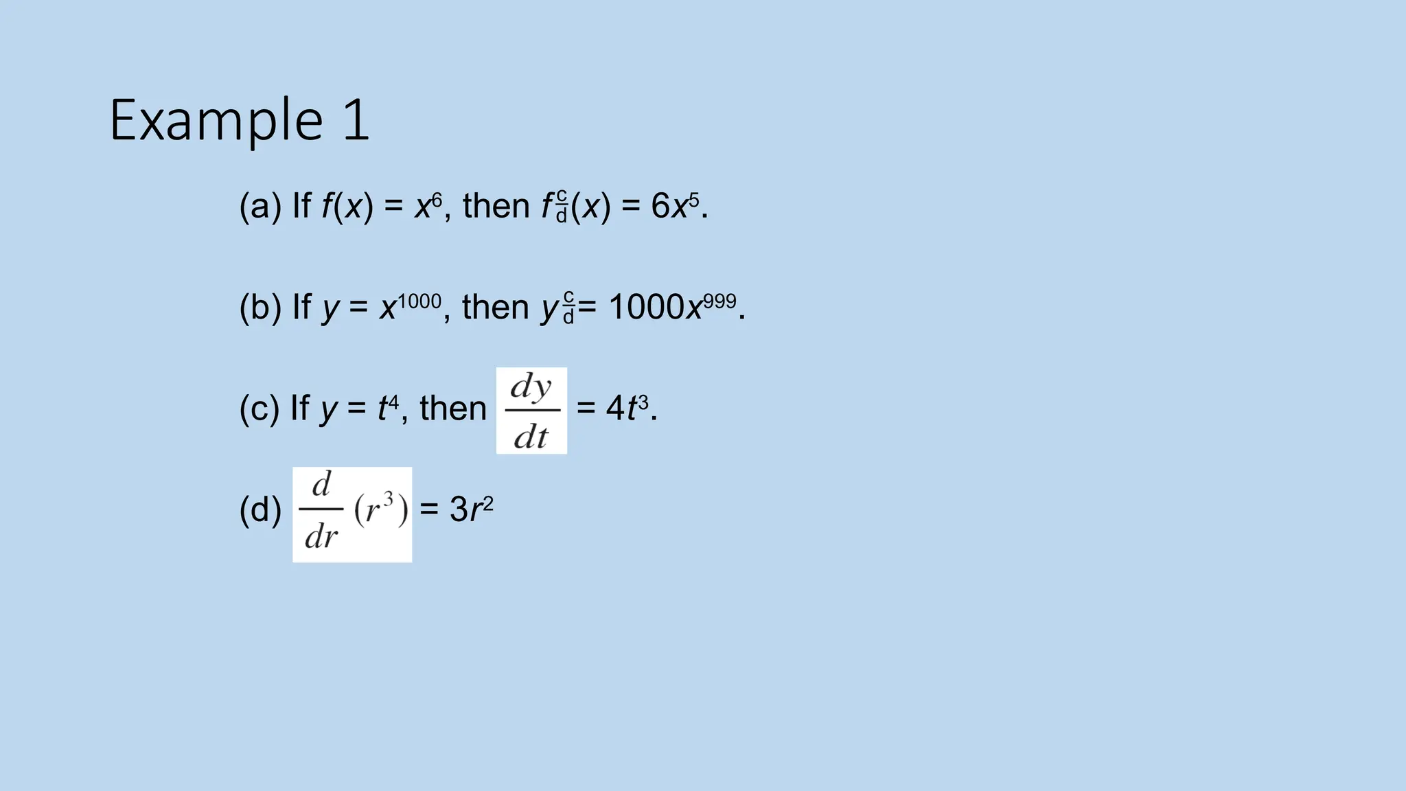
11. Example 1
(a) If f(x) = x6
, then f(x) = 6x5
.
(b) If y = x1000
, then y= 1000x999
.
(c) If y = t4
, then = 4t3
.
(d) = 3r2

12. Power Functions
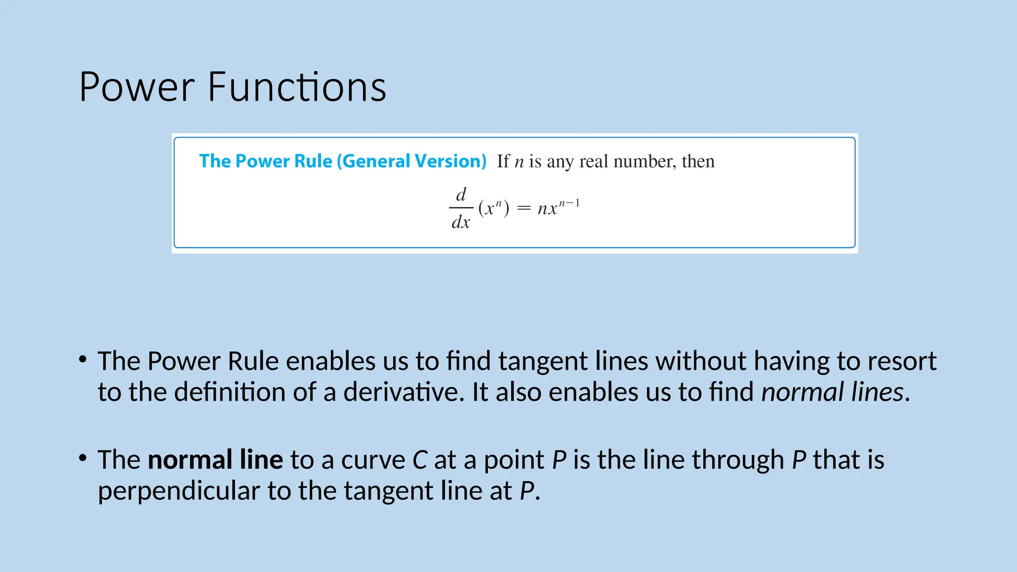
• The Power Rule enables us to find tangent lines without having to resort
to the definition of a derivative. It also enables us to find normal lines.
• The normal line to a curve C at a point P is the line through P that is
perpendicular to the tangent line at P.

13. New Derivatives from Old

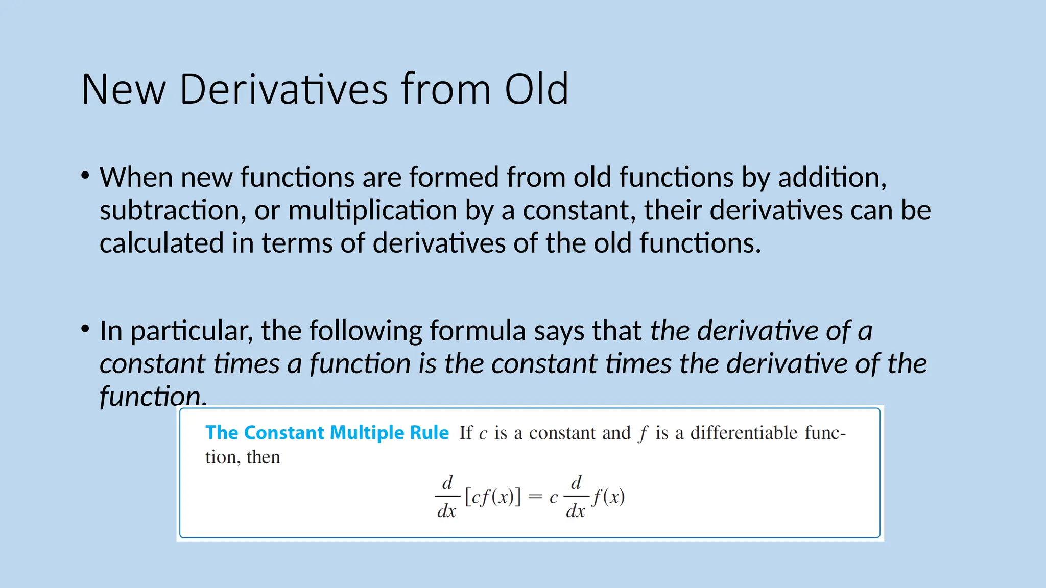
14. New Derivatives from Old
• When new functions are formed from old functions by addition,
subtraction, or multiplication by a constant, their derivatives can be
calculated in terms of derivatives of the old functions.
• In particular, the following formula says that the derivative of a
constant times a function is the constant times the derivative of the
function.

15. Example 4

16. New Derivatives from Old
• The next rule tells us that the derivative of a sum of functions is the sum of the derivatives.
• The Sum Rule can be extended to the sum of any number of functions. For instance, using
this theorem twice, we get
• (f + g + h) = [(f + g) + h)] = (f + g) + h = f + g + h

17. New Derivatives from Old
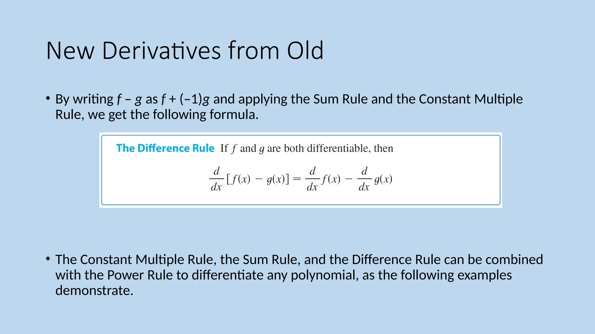
• By writing f – g as f + (–1)g and applying the Sum Rule and the Constant Multiple
Rule, we get the following formula.
• The Constant Multiple Rule, the Sum Rule, and the Difference Rule can be combined
with the Power Rule to differentiate any polynomial, as the following examples
demonstrate.

18. Exponential Functions

19. Exponential Functions
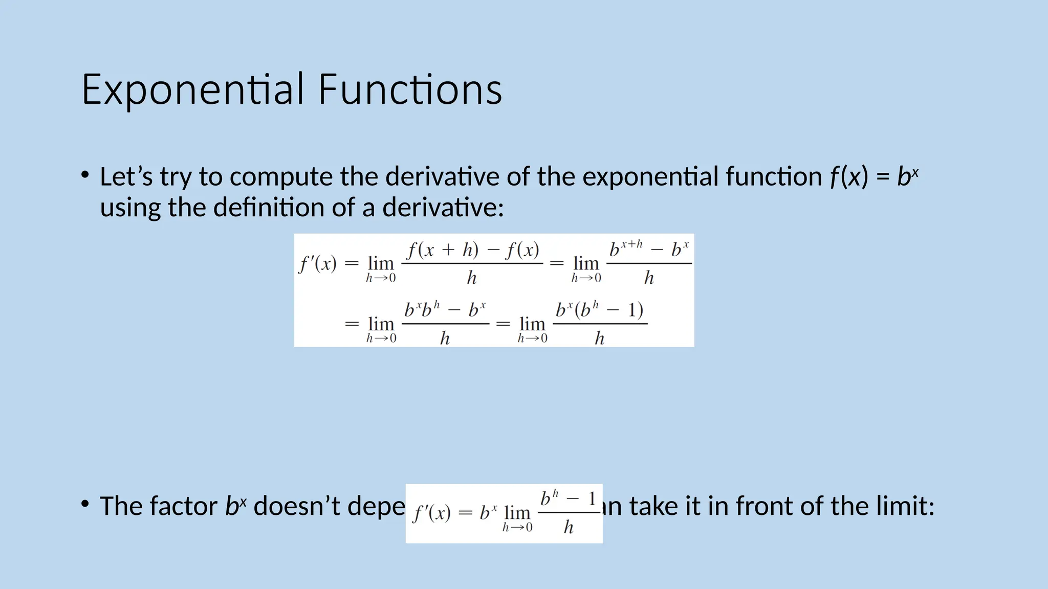
• Let’s try to compute the derivative of the exponential function f(x) = bx
using the definition of a derivative:
• The factor bx
doesn’t depend on h, so we can take it in front of the limit:

20. Exponential Functions
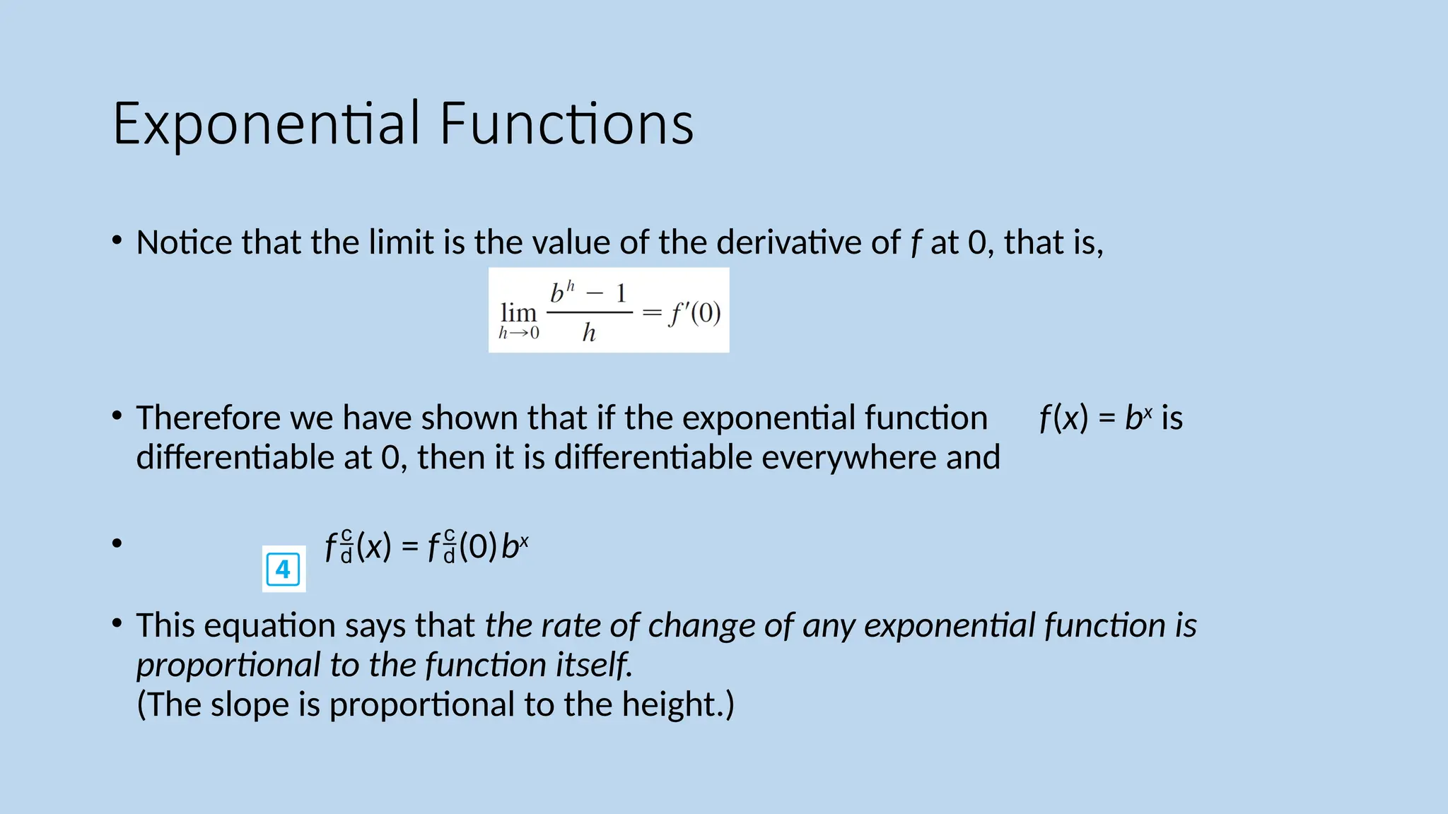
• Notice that the limit is the value of the derivative of f at 0, that is,
• Therefore we have shown that if the exponential function f(x) = bx
is
differentiable at 0, then it is differentiable everywhere and
• f(x) = f(0)bx
• This equation says that the rate of change of any exponential function is
proportional to the function itself.
(The slope is proportional to the height.)

21. Exponential Functions
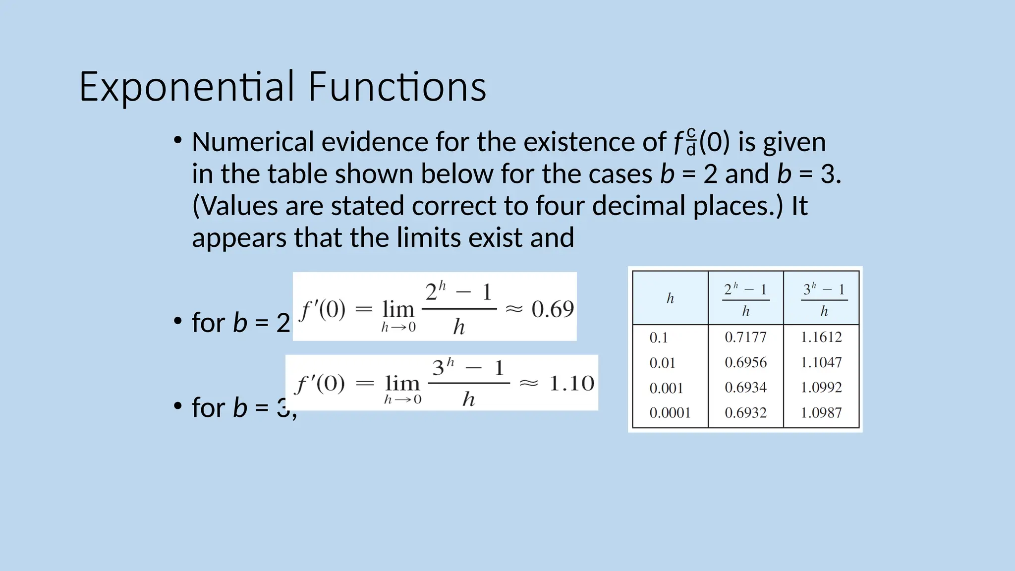
• Numerical evidence for the existence of f(0) is given
in the table shown below for the cases b = 2 and b = 3.
(Values are stated correct to four decimal places.) It
appears that the limits exist and
• for b = 2,
• for b = 3,

22. Exponential Functions
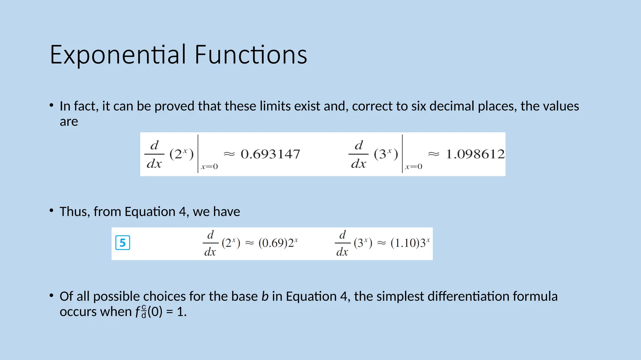
• In fact, it can be proved that these limits exist and, correct to six decimal places, the values
are
• Thus, from Equation 4, we have
• Of all possible choices for the base b in Equation 4, the simplest differentiation formula
occurs when f(0) = 1.

23. Exponential Functions
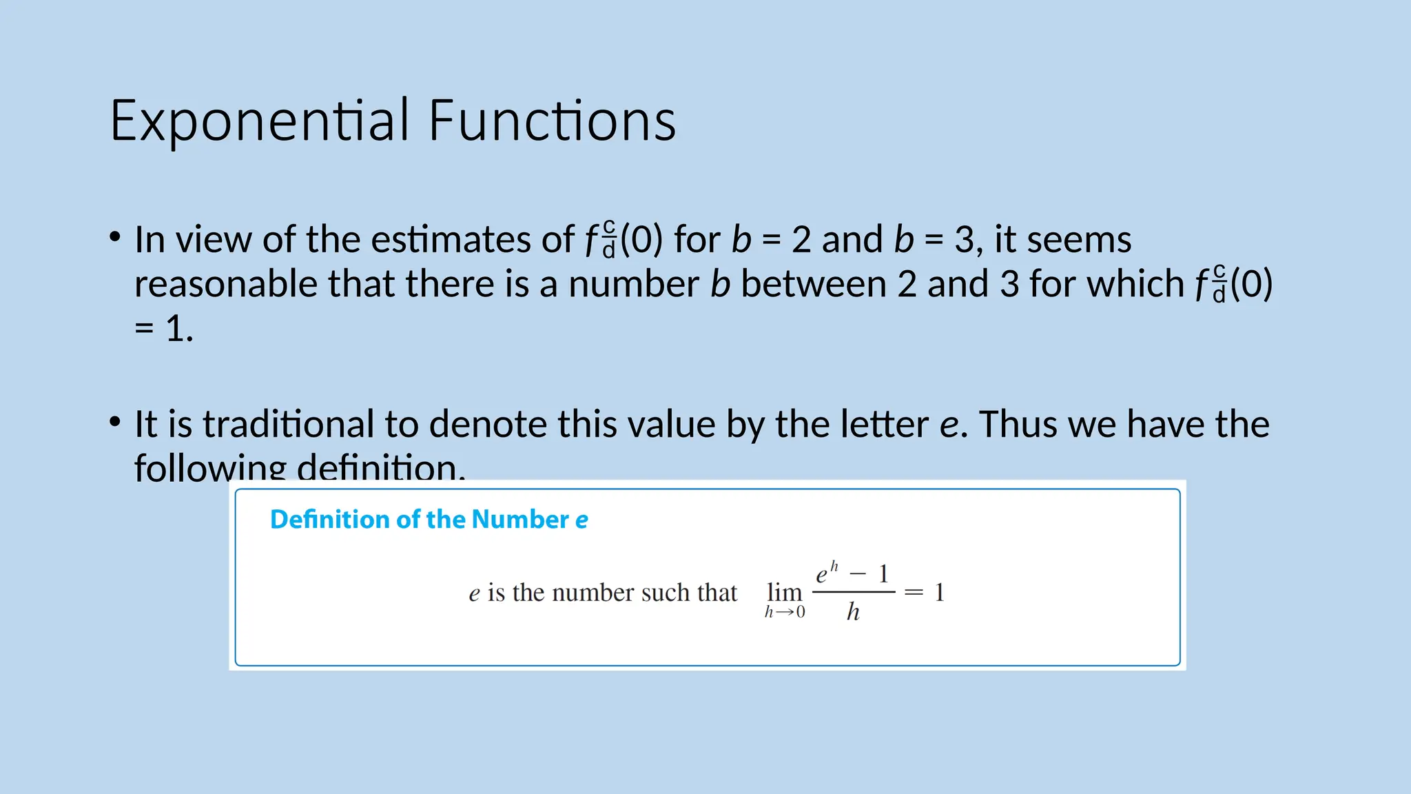
• In view of the estimates of f(0) for b = 2 and b = 3, it seems
reasonable that there is a number b between 2 and 3 for which f(0)
= 1.
• It is traditional to denote this value by the letter e. Thus we have the
following definition.

24. Exponential Functions
• Geometrically, this means that of all the possible exponential
functions y = bx
, the function f(x) = ex
is the one whose tangent line at
(0, 1) has a slope f(0) that is
exactly 1. (See Figures 6 and 7.)
Figure 6 Figure 7

25. Exponential Functions
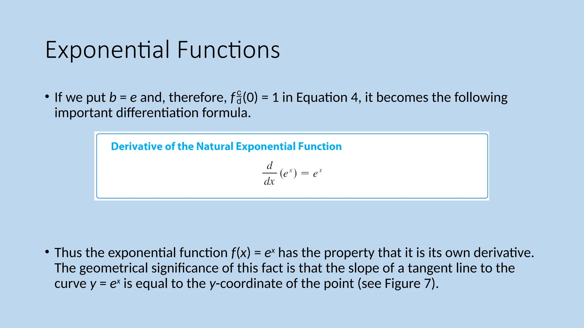
• If we put b = e and, therefore, f(0) = 1 in Equation 4, it becomes the following
important differentiation formula.
• Thus the exponential function f(x) = ex
has the property that it is its own derivative.
The geometrical significance of this fact is that the slope of a tangent line to the
curve y = ex
is equal to the y-coordinate of the point (see Figure 7).

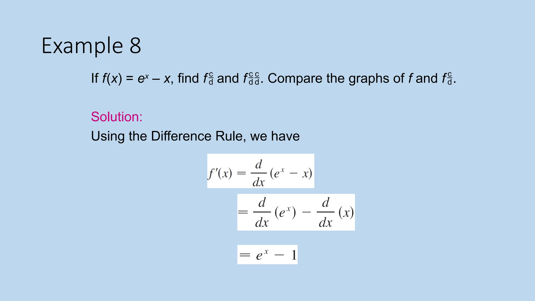
26. Example 8
If f(x) = ex
– x, find f and f. Compare the graphs of f and f.
Solution:
Using the Difference Rule, we have

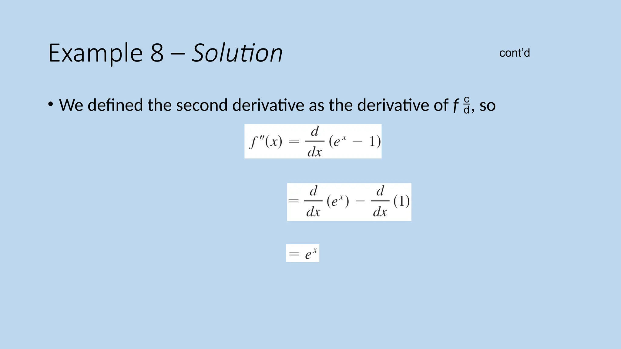
27. Example 8 – Solution
• We defined the second derivative as the derivative of f , so
cont’d

28. Example 8 – Solution
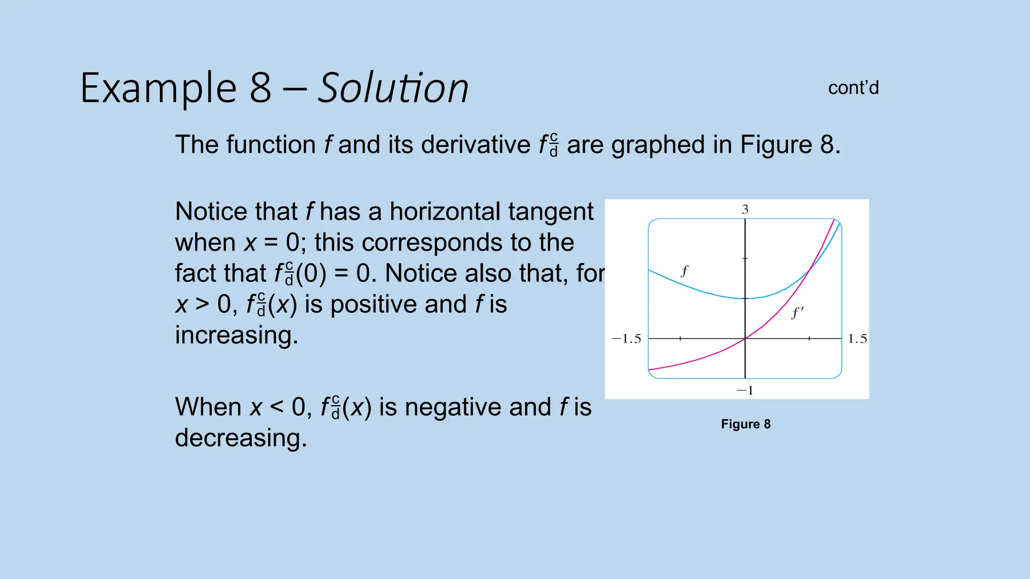
The function f and its derivative f are graphed in Figure 8.
Notice that f has a horizontal tangent
when x = 0; this corresponds to the
fact that f(0) = 0. Notice also that, for
x > 0, f(x) is positive and f is
increasing.
When x < 0, f(x) is negative and f is
decreasing.
Figure 8
cont’d

29. The Product and Quotient
Rules

30. The Product Rule

31. The Product Rule
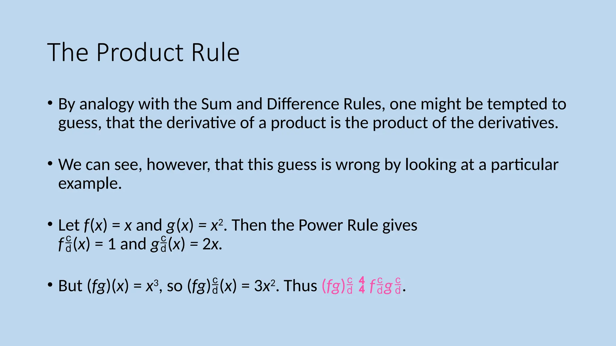
• By analogy with the Sum and Difference Rules, one might be tempted to
guess, that the derivative of a product is the product of the derivatives.
• We can see, however, that this guess is wrong by looking at a particular
example.
• Let f(x) = x and g(x) = x2
. Then the Power Rule gives
f(x) = 1 and g(x) = 2x.
• But (fg)(x) = x3
, so (fg)(x) = 3x2
. Thus (fg)  fg.

32. The Product Rule
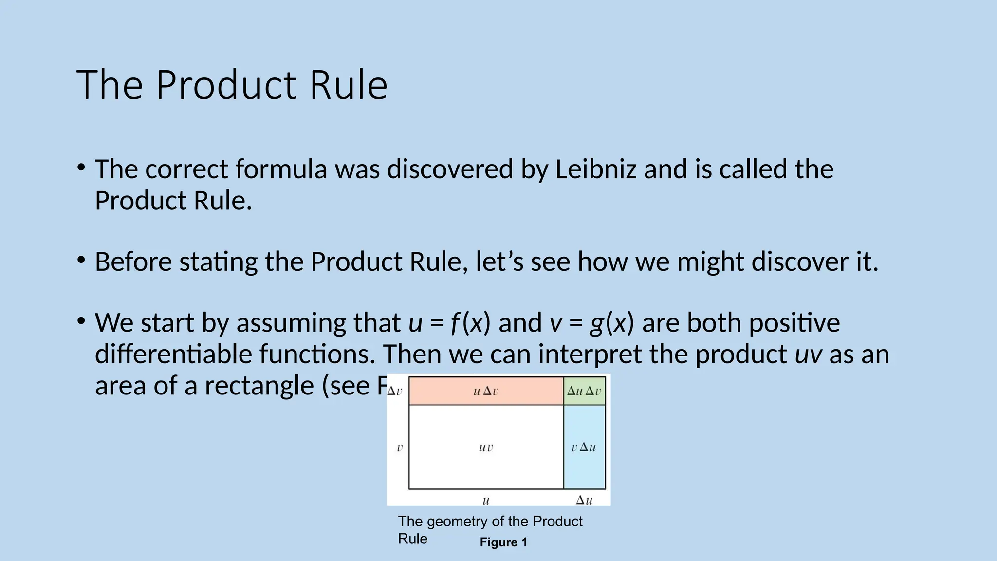
• The correct formula was discovered by Leibniz and is called the
Product Rule.
• Before stating the Product Rule, let’s see how we might discover it.
• We start by assuming that u = f(x) and v = g(x) are both positive
differentiable functions. Then we can interpret the product uv as an
area of a rectangle (see Figure 1).
Figure 1
The geometry of the Product
Rule

33. The Product Rule
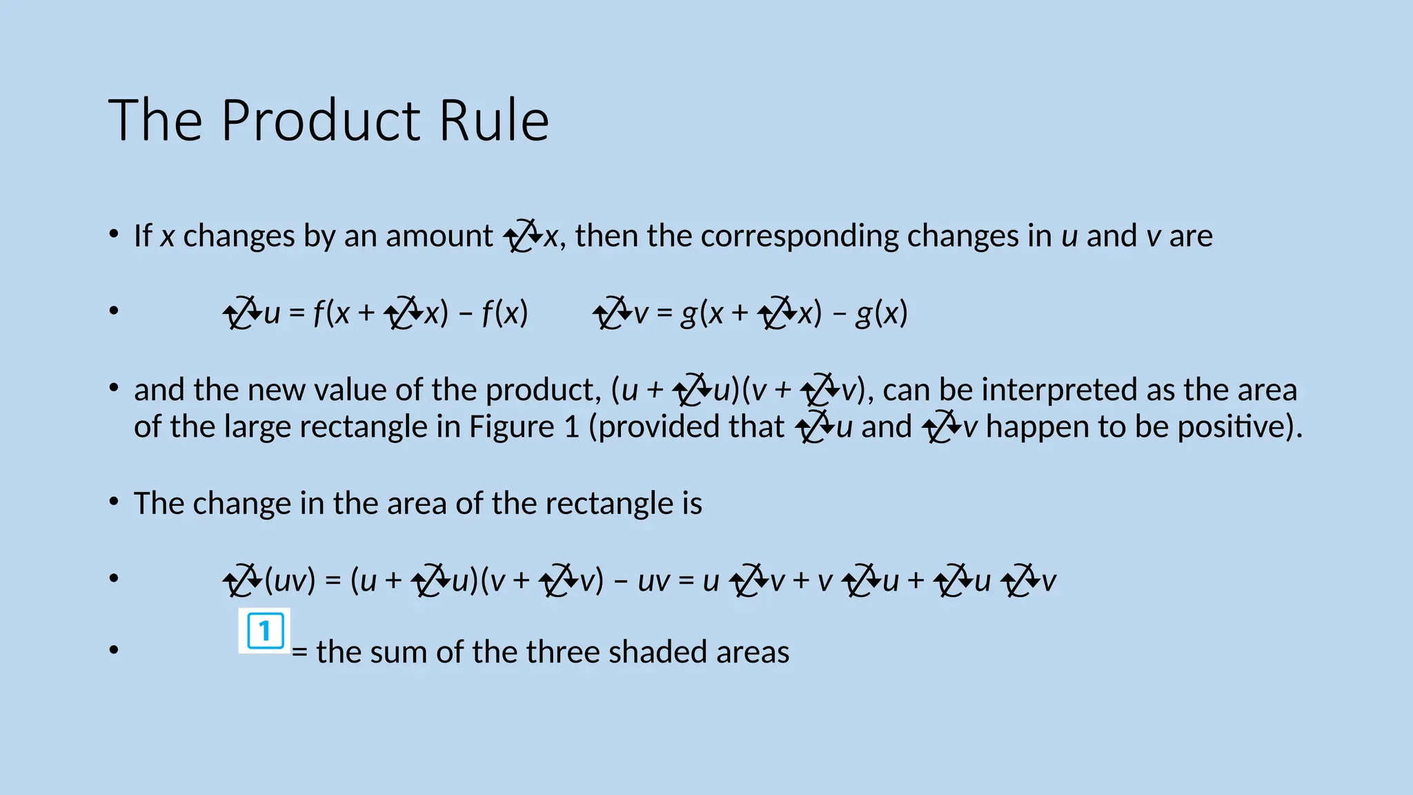
• If x changes by an amount x, then the corresponding changes in u and v are
• u = f(x + x) – f(x) v = g(x + x) – g(x)
• and the new value of the product, (u + u)(v + v), can be interpreted as the area
of the large rectangle in Figure 1 (provided that u and v happen to be positive).
• The change in the area of the rectangle is
• (uv) = (u + u)(v + v) – uv = u v + v u + u v
• = the sum of the three shaded areas

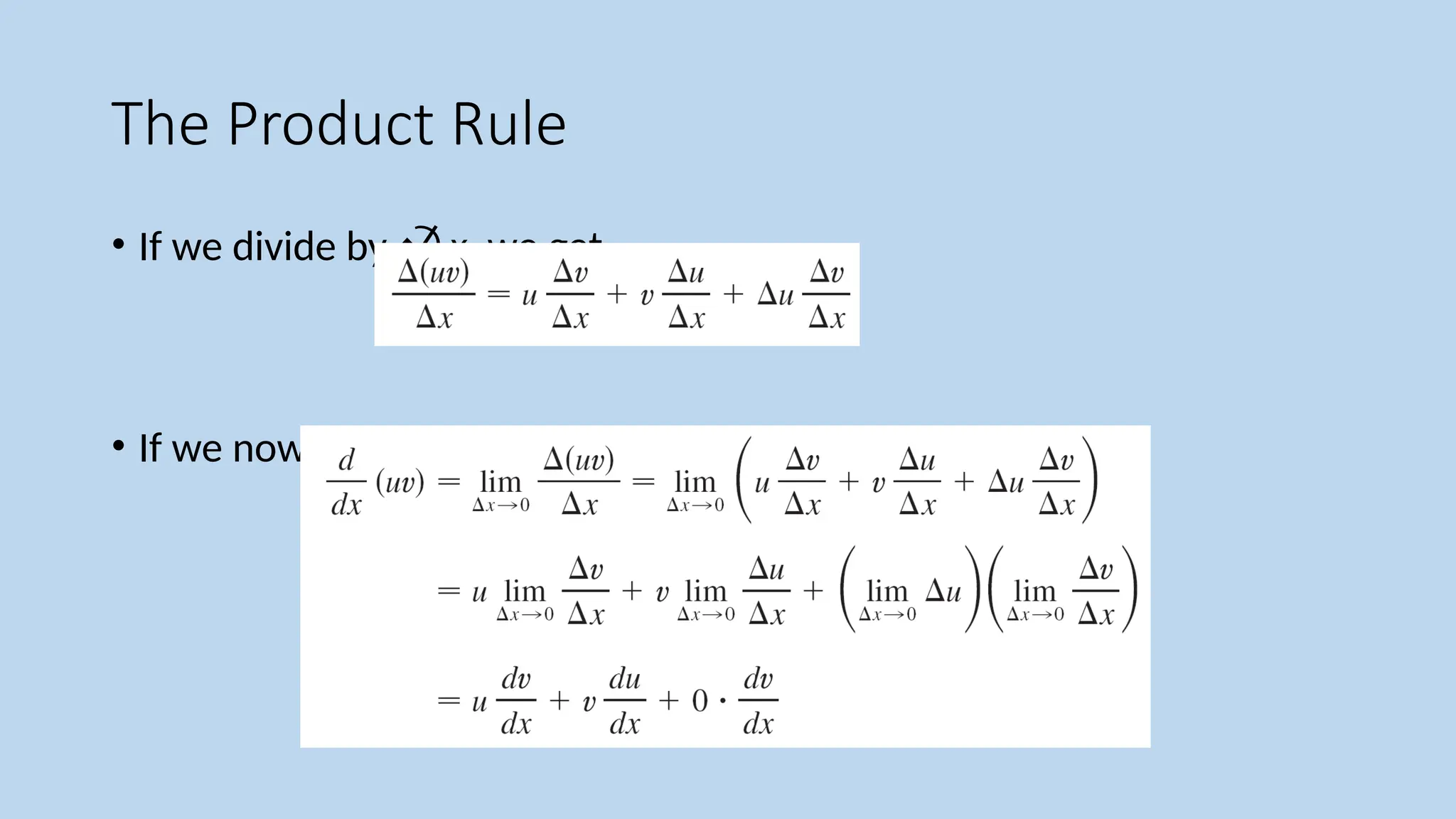
34. • If we divide by x, we get
• If we now let x  0, we get the derivative of uv:
The Product Rule

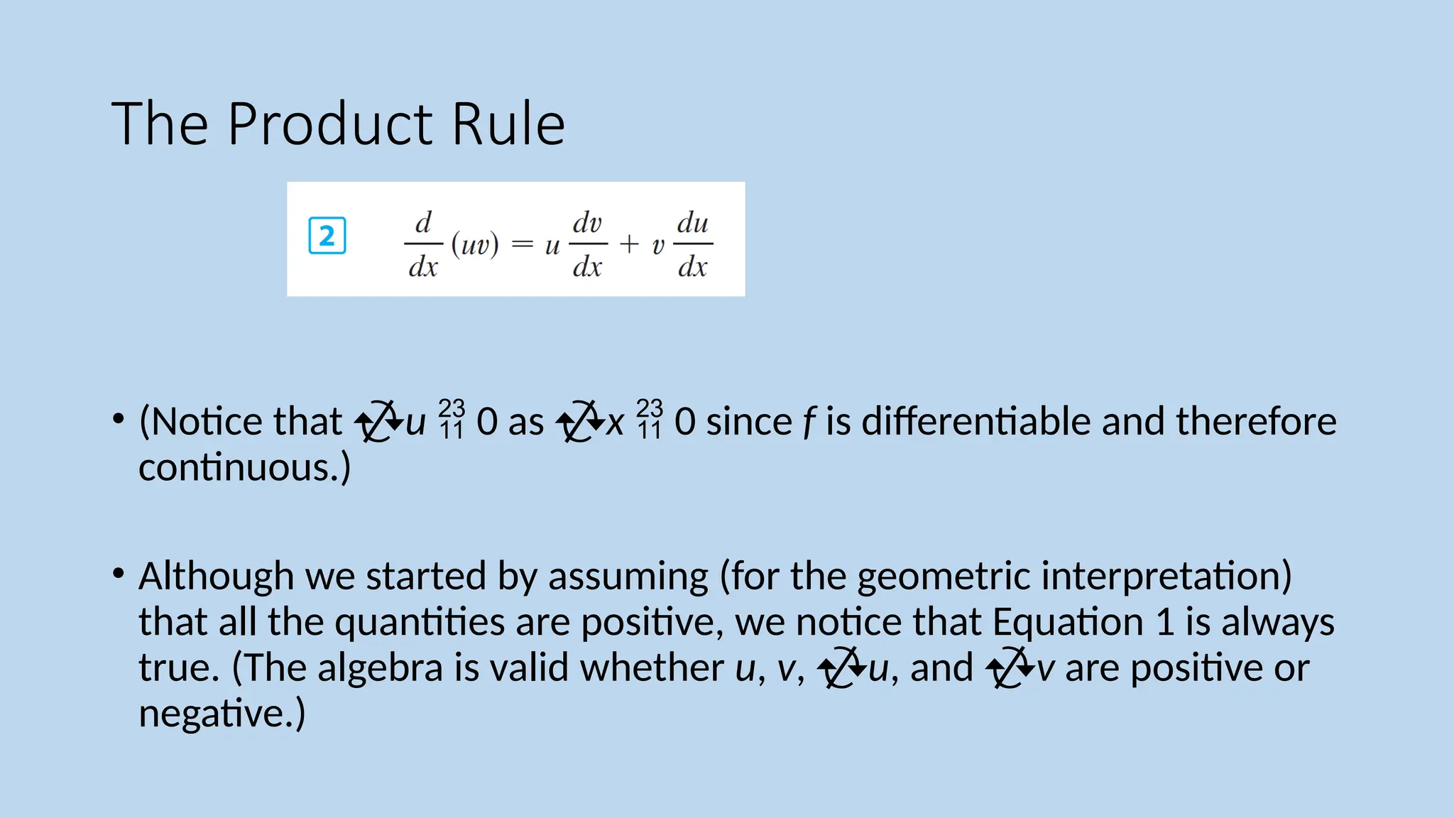
35. The Product Rule
• (Notice that u  0 as x  0 since f is differentiable and therefore
continuous.)
• Although we started by assuming (for the geometric interpretation)
that all the quantities are positive, we notice that Equation 1 is always
true. (The algebra is valid whether u, v, u, and v are positive or
negative.)

36. The Product Rule
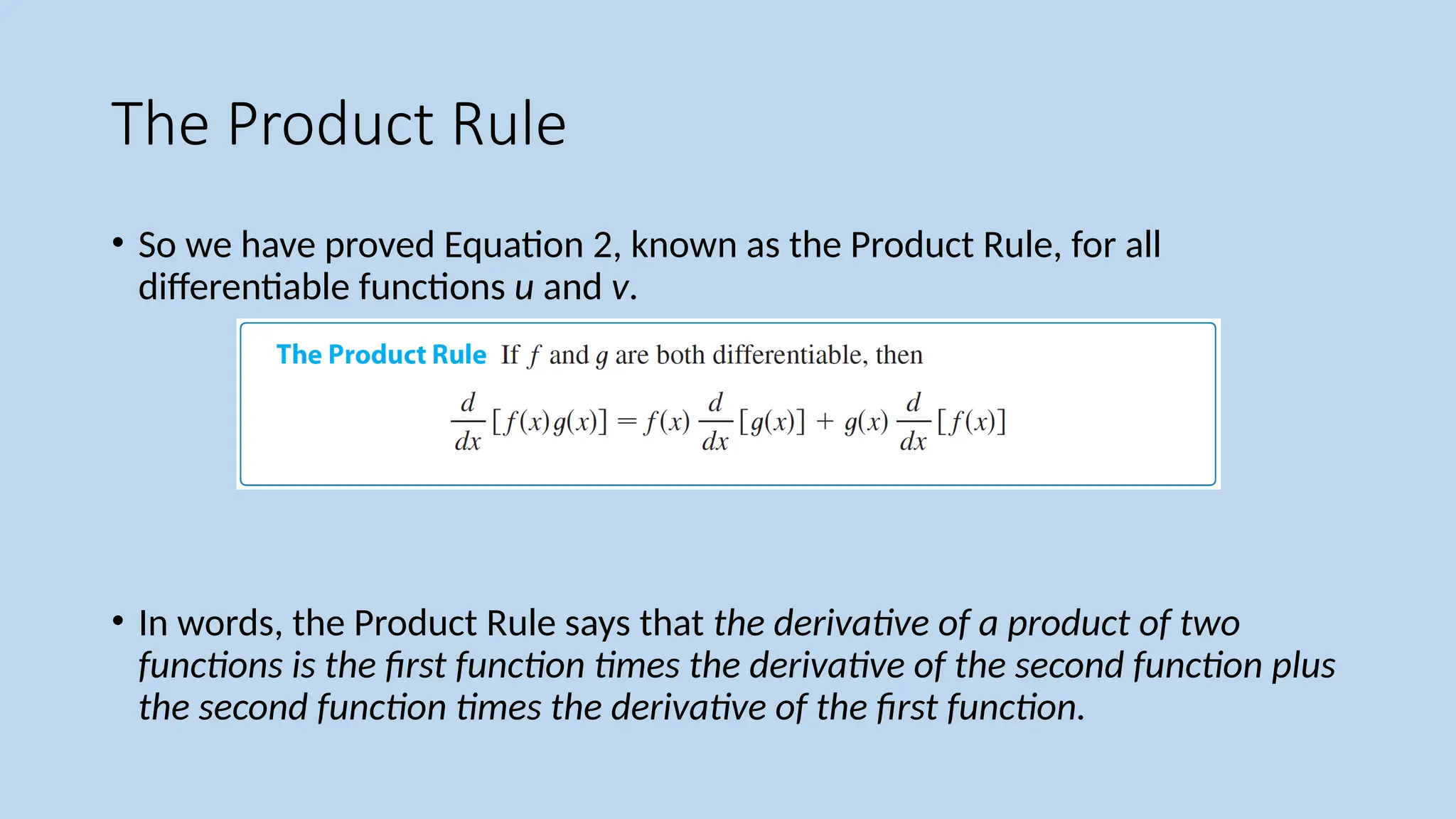
• So we have proved Equation 2, known as the Product Rule, for all
differentiable functions u and v.
• In words, the Product Rule says that the derivative of a product of two
functions is the first function times the derivative of the second function plus
the second function times the derivative of the first function.

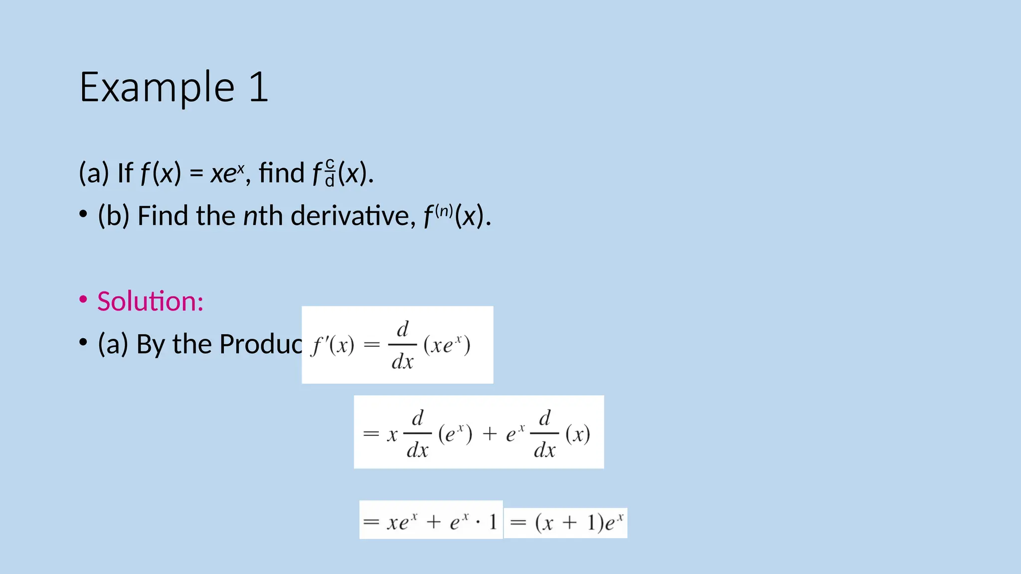
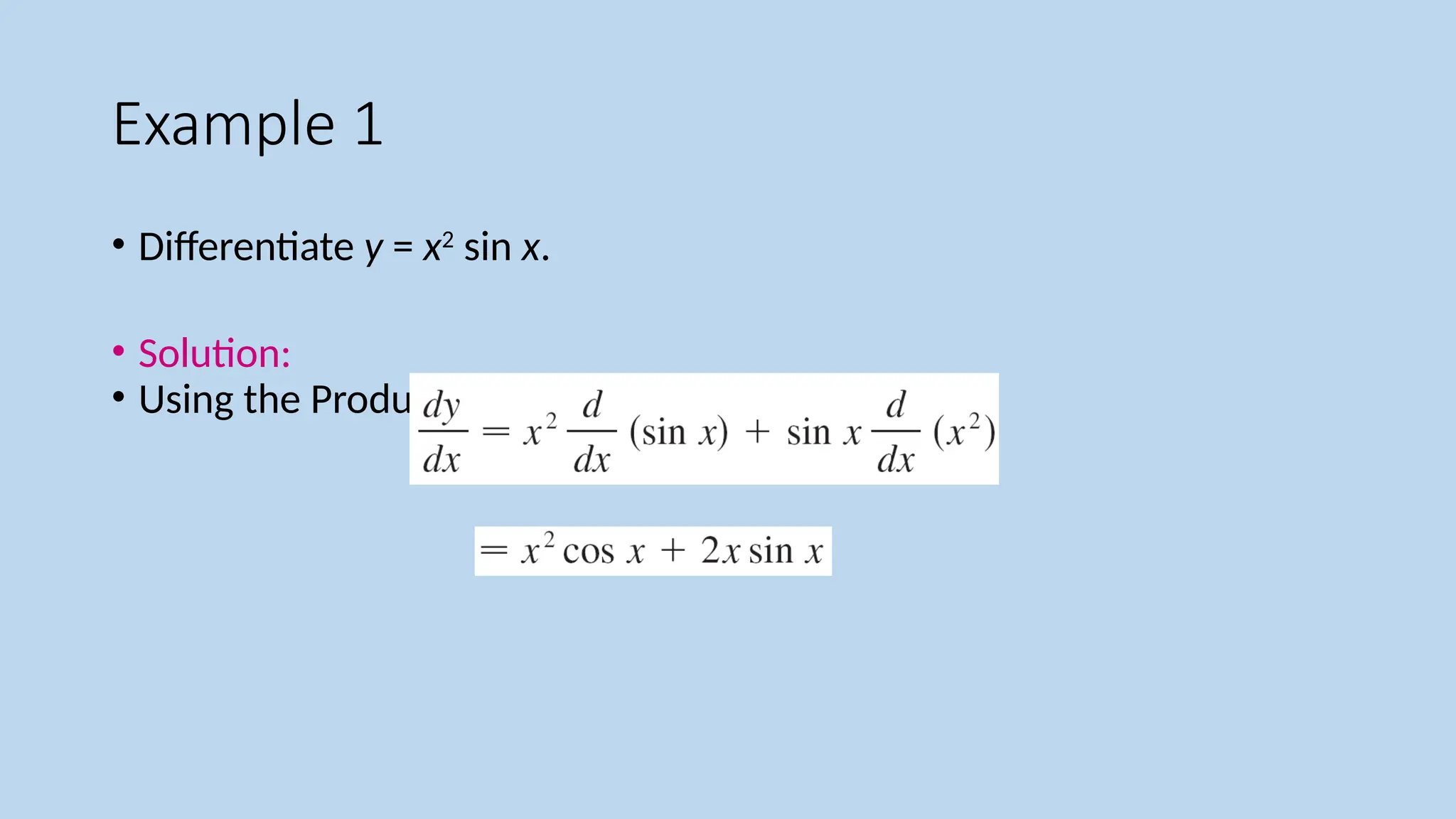
37. Example 1
(a) If f(x) = xex
, find f(x).
• (b) Find the nth derivative, f(n)
(x).
• Solution:
• (a) By the Product Rule, we have

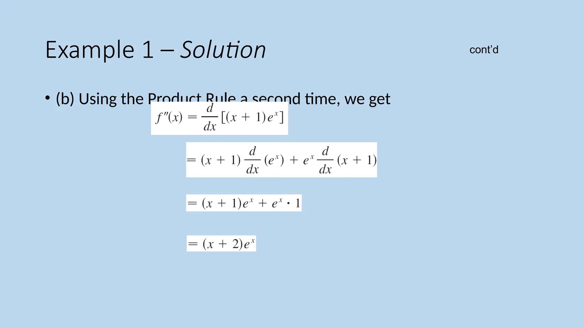
38. Example 1 – Solution
• (b) Using the Product Rule a second time, we get
cont’d

39. Example 1 – Solution
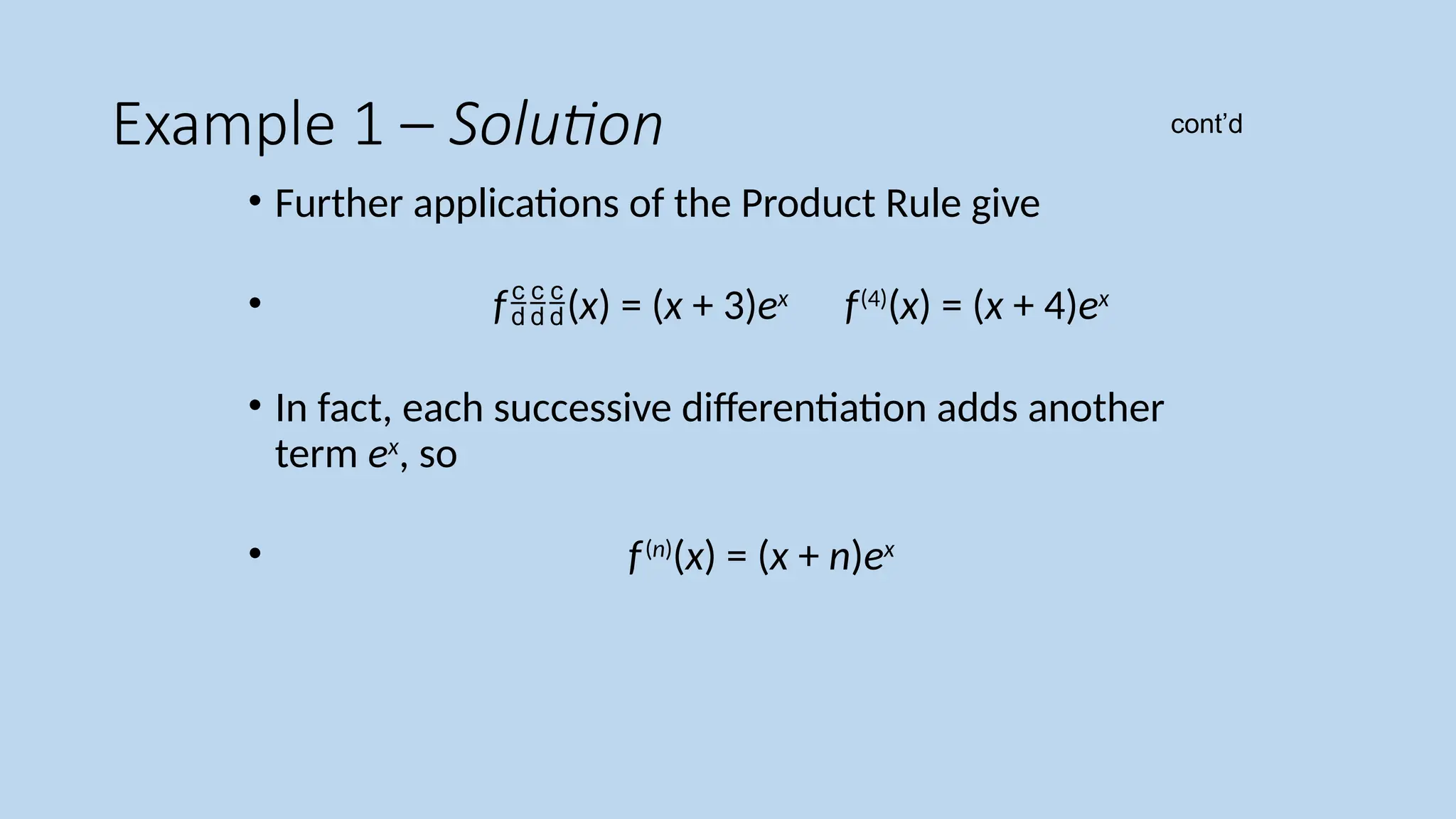
• Further applications of the Product Rule give
• f(x) = (x + 3)ex
f(4)
(x) = (x + 4)ex
• In fact, each successive differentiation adds another
term ex
, so
• f(n)
(x) = (x + n)ex
cont’d

40. The Quotient Rule

41. The Quotient Rule
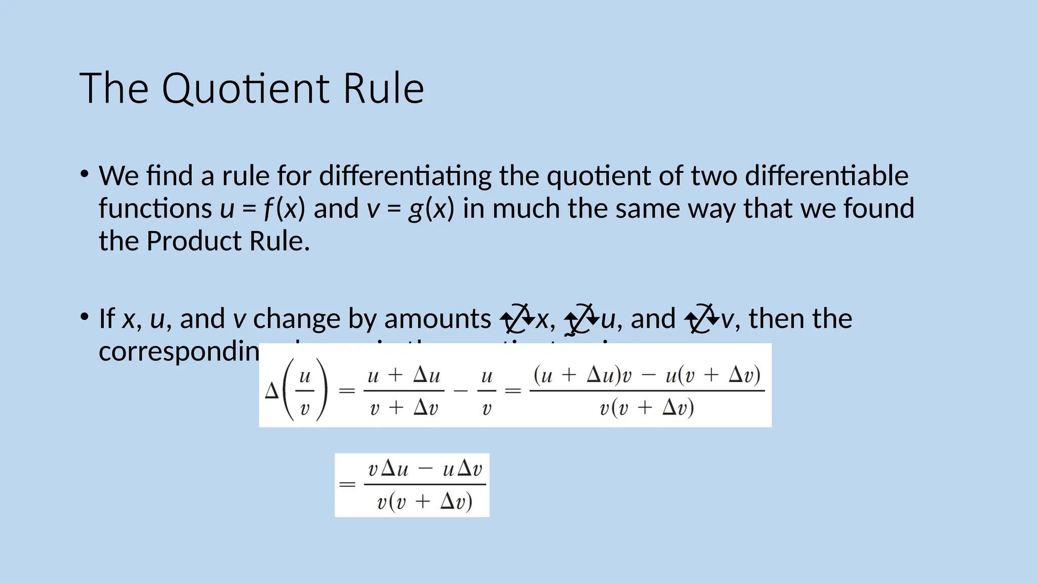
• We find a rule for differentiating the quotient of two differentiable
functions u = f(x) and v = g(x) in much the same way that we found
the Product Rule.
• If x, u, and v change by amounts x, u, and v, then the
corresponding change in the quotient uv is

42. The Quotient Rule
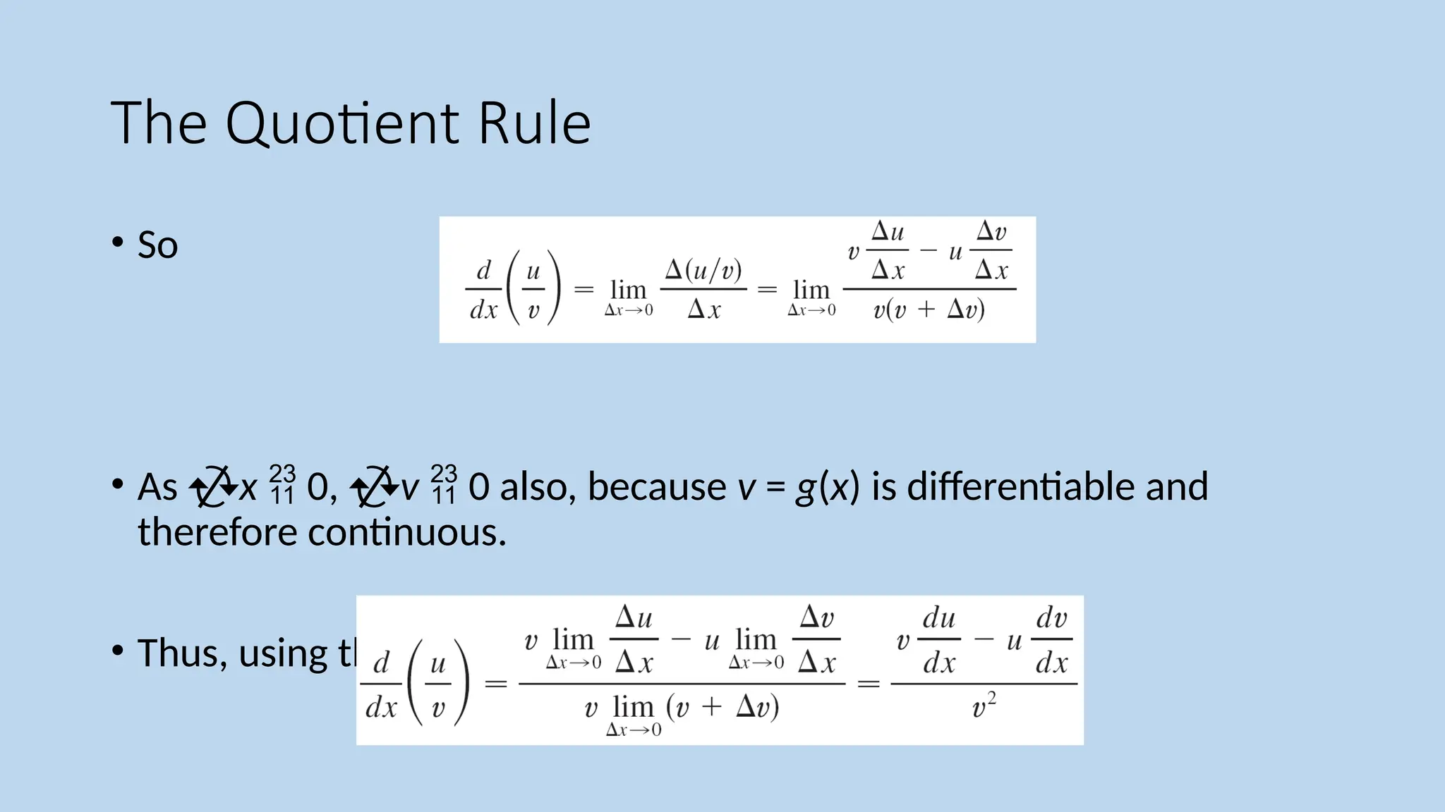
• So
• As x  0, v  0 also, because v = g(x) is differentiable and
therefore continuous.
• Thus, using the Limit Laws, we get

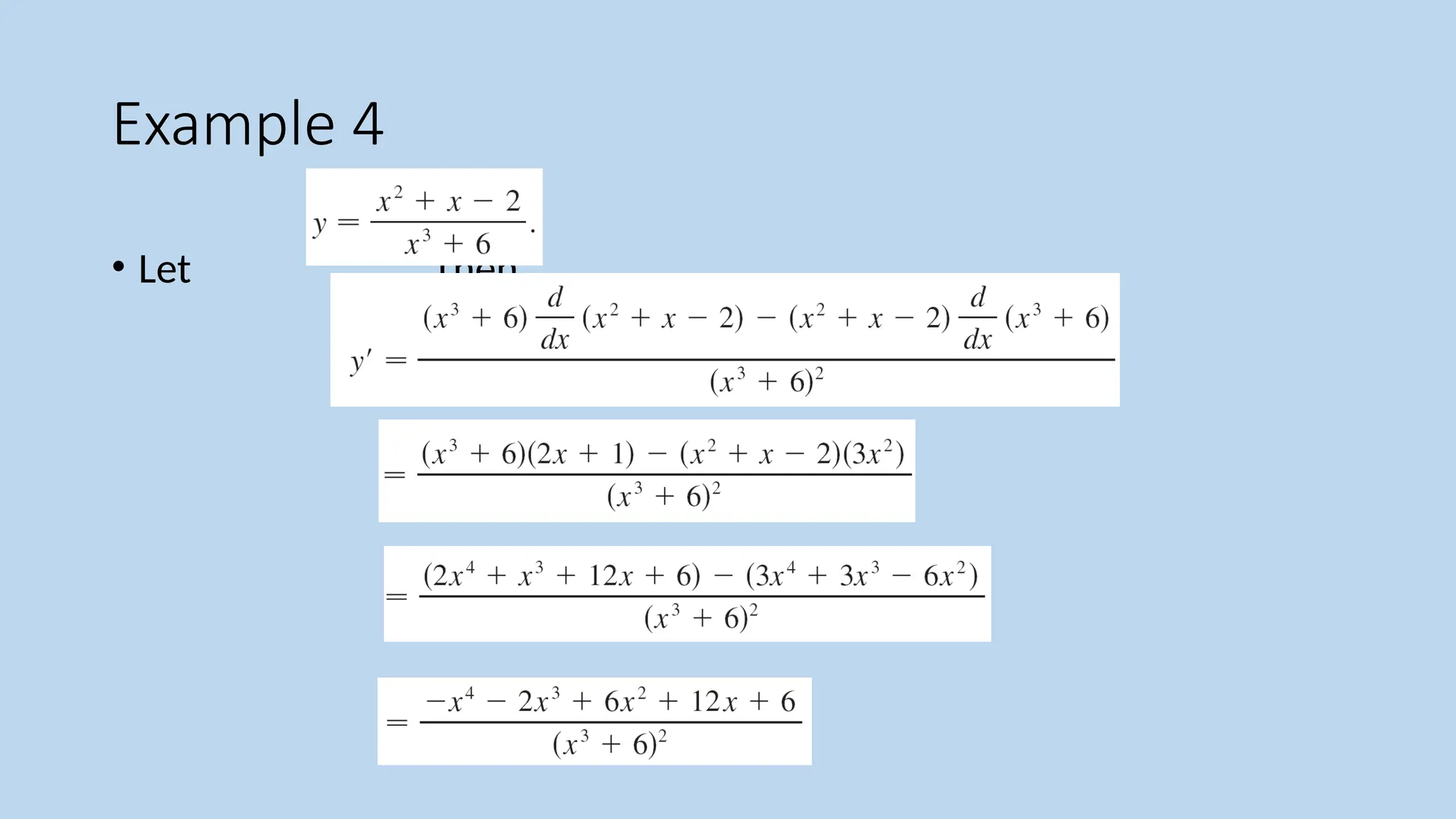
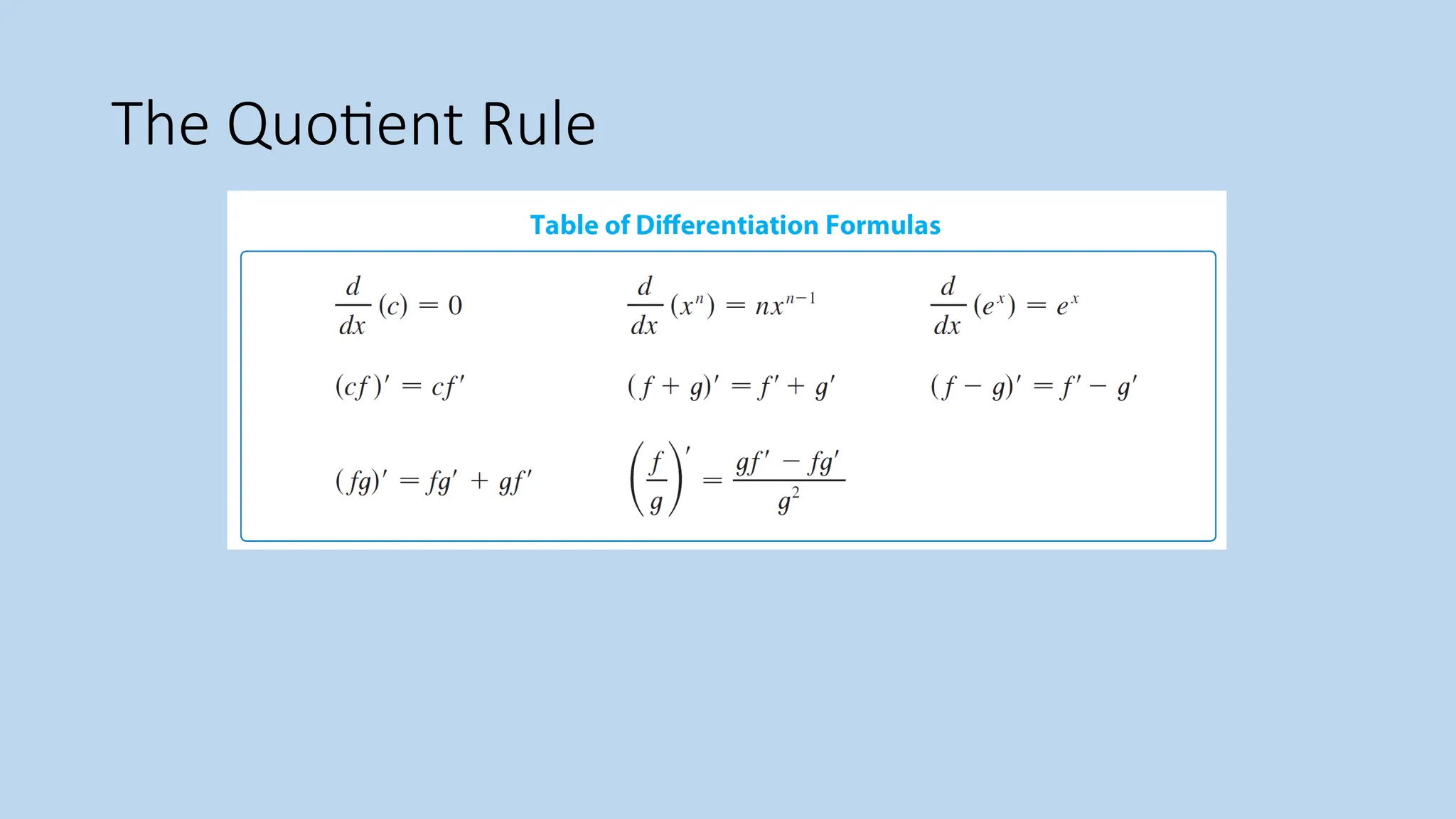
43. The Quotient Rule
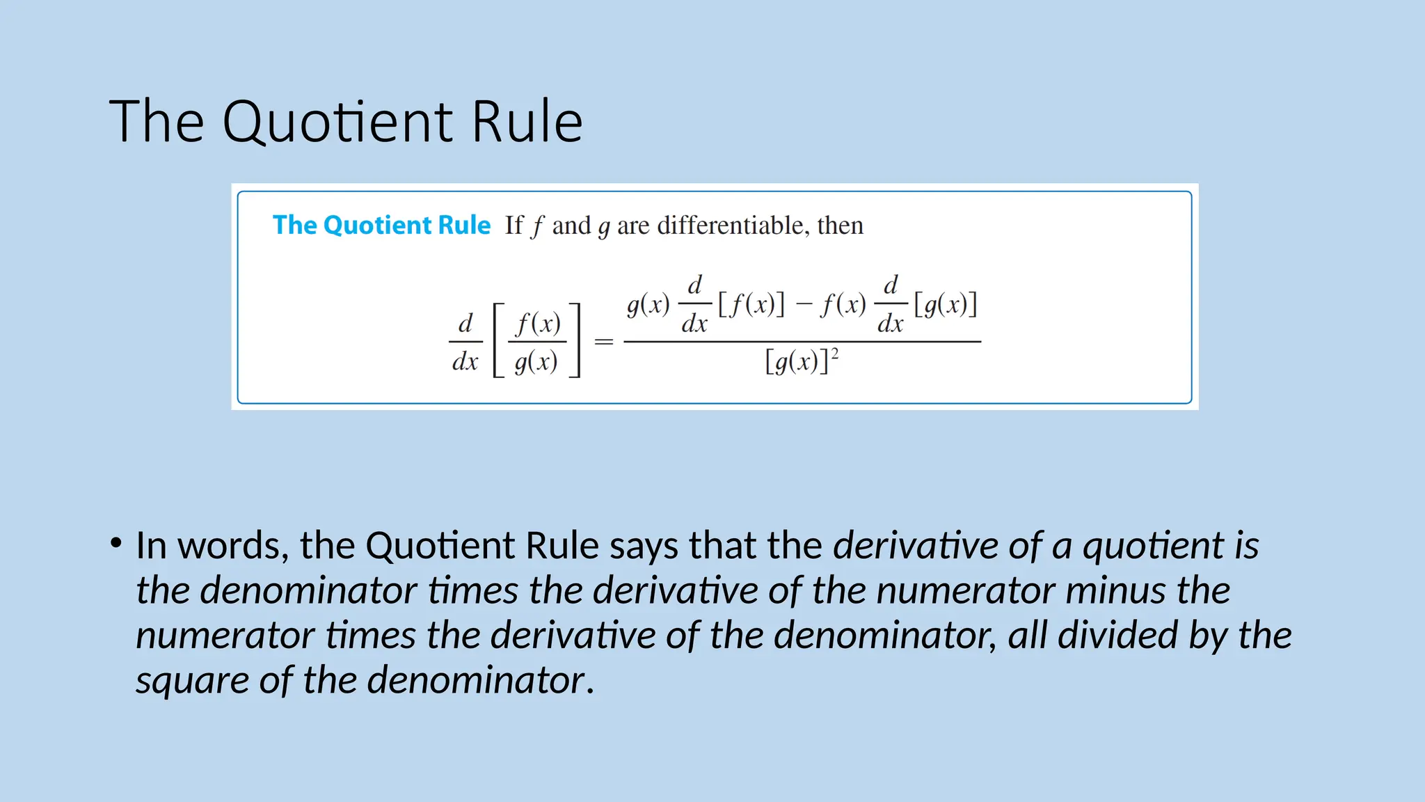
• In words, the Quotient Rule says that the derivative of a quotient is
the denominator times the derivative of the numerator minus the
numerator times the derivative of the denominator, all divided by the
square of the denominator.

44. Example 4
• Let Then

45. The Quotient Rule

46. Derivatives of Trigonometric
Functions

47. Derivatives of Trigonometric Functions
• In particular, it is important to remember that when we talk about the
function f defined for all real numbers x by
• f(x) = sin x
• it is understood that sin x means the sine of the angle whose radian
measure is x. A similar convention holds for the other trigonometric
functions cos, tan, csc, sec, and cot.
• All of the trigonometric functions are continuous at every number in their
domains.

48. Derivatives of Trigonometric Functions
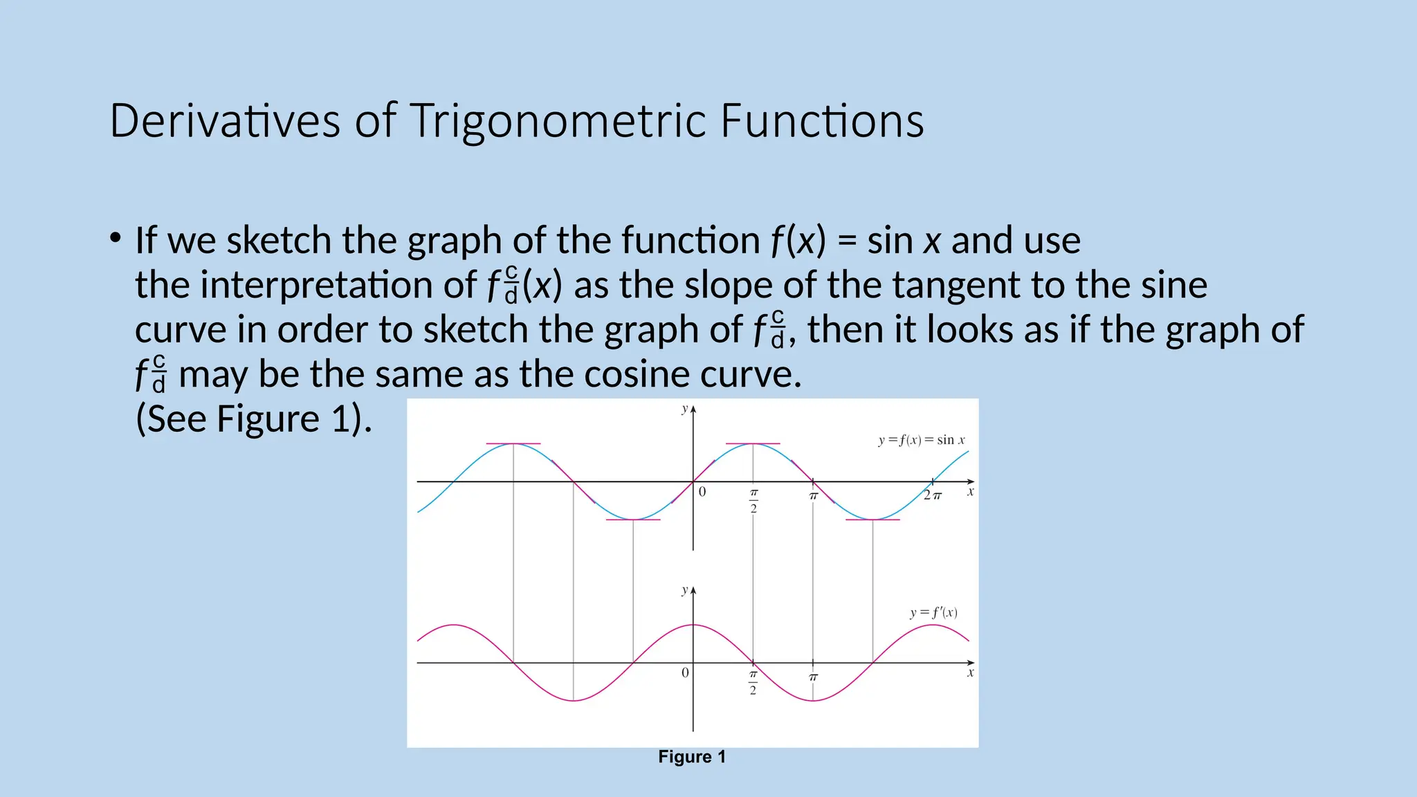
• If we sketch the graph of the function f(x) = sin x and use
the interpretation of f(x) as the slope of the tangent to the sine
curve in order to sketch the graph of f, then it looks as if the graph of
f may be the same as the cosine curve.
(See Figure 1).
Figure 1

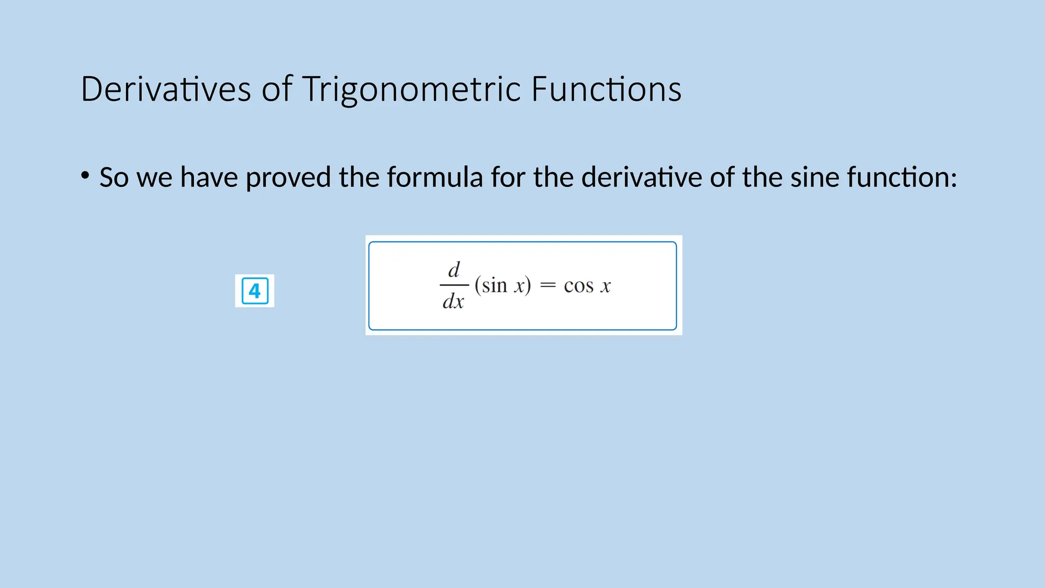
49. Derivatives of Trigonometric Functions
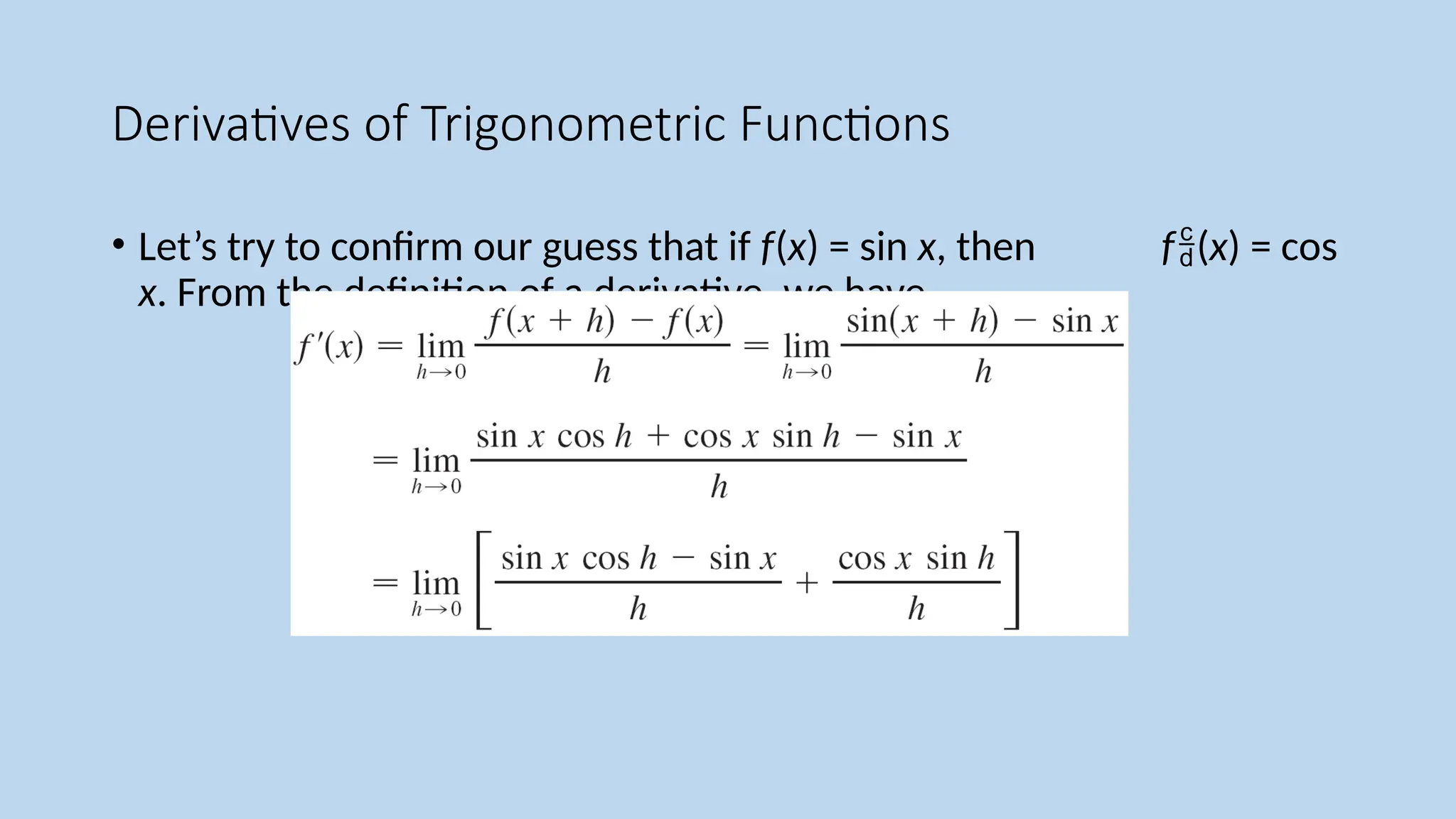
• Let’s try to confirm our guess that if f(x) = sin x, then f(x) = cos
x. From the definition of a derivative, we have

50. Derivatives of Trigonometric Functions
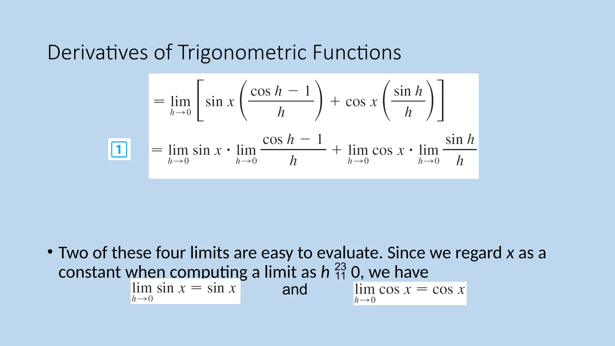
• Two of these four limits are easy to evaluate. Since we regard x as a
constant when computing a limit as h  0, we have
and

51. Derivatives of Trigonometric Functions
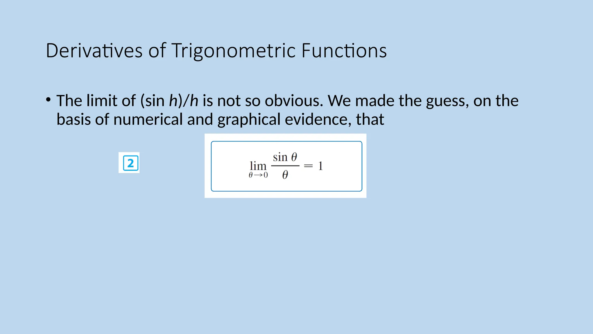
• The limit of (sin h)/h is not so obvious. We made the guess, on the
basis of numerical and graphical evidence, that

52. Derivatives of Trigonometric Functions
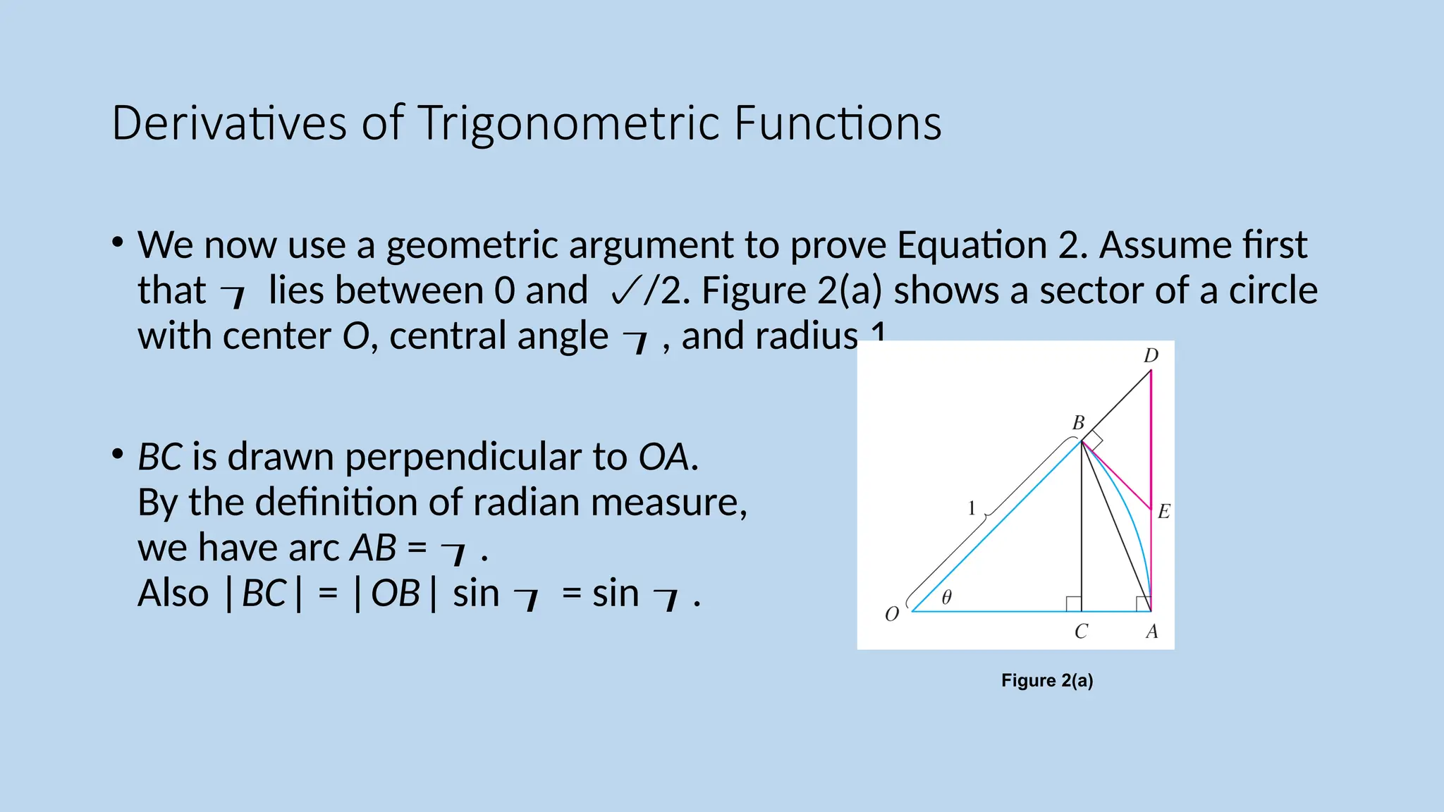
• We now use a geometric argument to prove Equation 2. Assume first
that  lies between 0 and /2. Figure 2(a) shows a sector of a circle
with center O, central angle , and radius 1.
• BC is drawn perpendicular to OA.
By the definition of radian measure,
we have arc AB = .
Also |BC| = |OB| sin  = sin .
Figure 2(a)

53. Derivatives of Trigonometric Functions
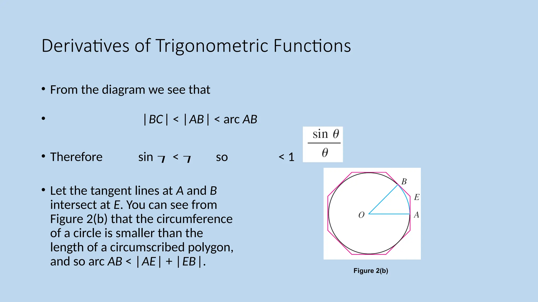
• From the diagram we see that
• |BC| < |AB| < arc AB
• Therefore sin  <  so < 1
• Let the tangent lines at A and B
intersect at E. You can see from
Figure 2(b) that the circumference
of a circle is smaller than the
length of a circumscribed polygon,
and so arc AB < |AE| + |EB|.
Figure 2(b)

54. Derivatives of Trigonometric Functions
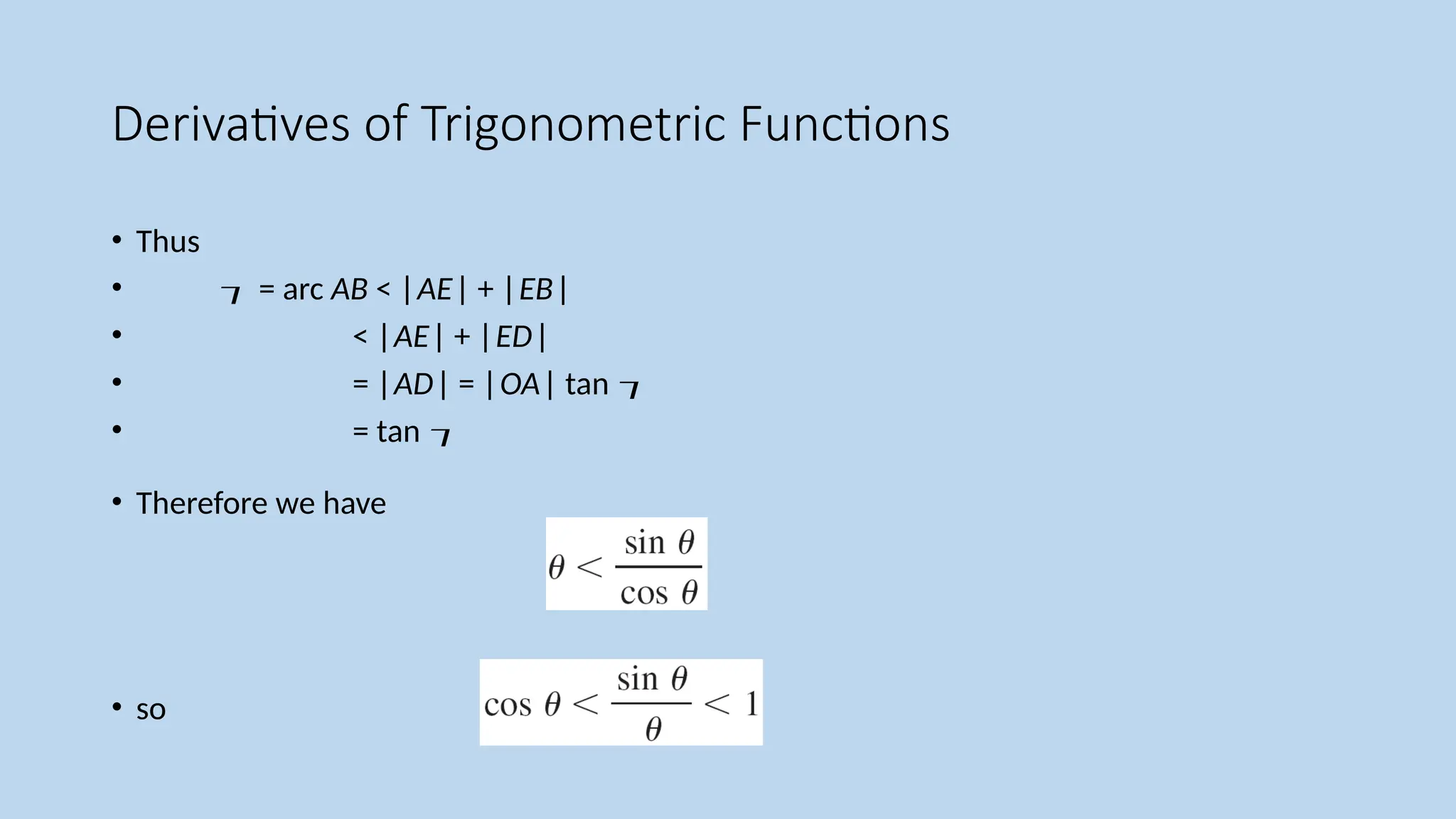
• Thus
•  = arc AB < |AE| + |EB|
• < |AE| + |ED|
• = |AD| = |OA| tan 
• = tan 
• Therefore we have
• so

55. Derivatives of Trigonometric Functions
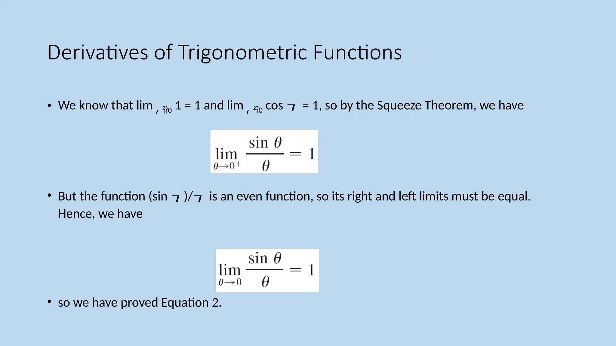
• We know that lim 0 1 = 1 and lim 0 cos  = 1, so by the Squeeze Theorem, we have
• But the function (sin )/ is an even function, so its right and left limits must be equal.
Hence, we have
• so we have proved Equation 2.

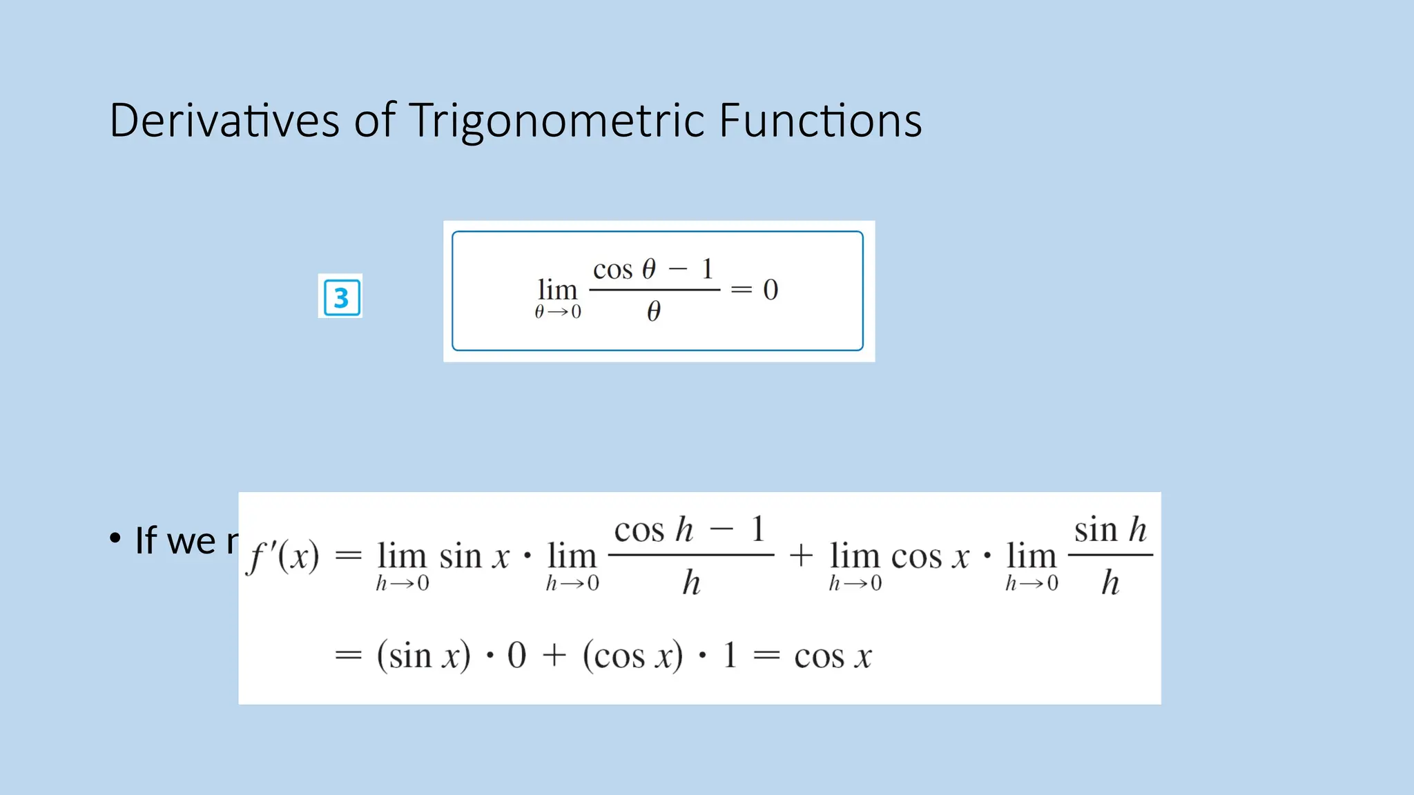
56. Derivatives of Trigonometric Functions
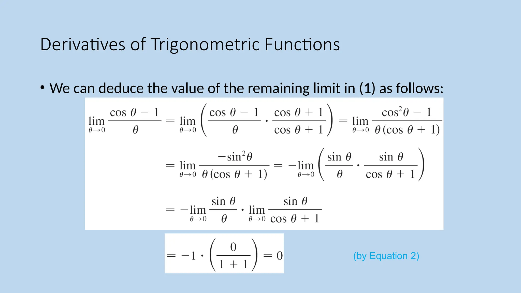
• We can deduce the value of the remaining limit in (1) as follows:
(by Equation 2)

57. Derivatives of Trigonometric Functions
• If we now put the limits (2) and (3) in (1), we get

58. Derivatives of Trigonometric Functions
• So we have proved the formula for the derivative of the sine function:

59. Example 1
• Differentiate y = x2
sin x.
• Solution:
• Using the Product Rule and Formula 4, we have

60. Derivatives of Trigonometric Functions
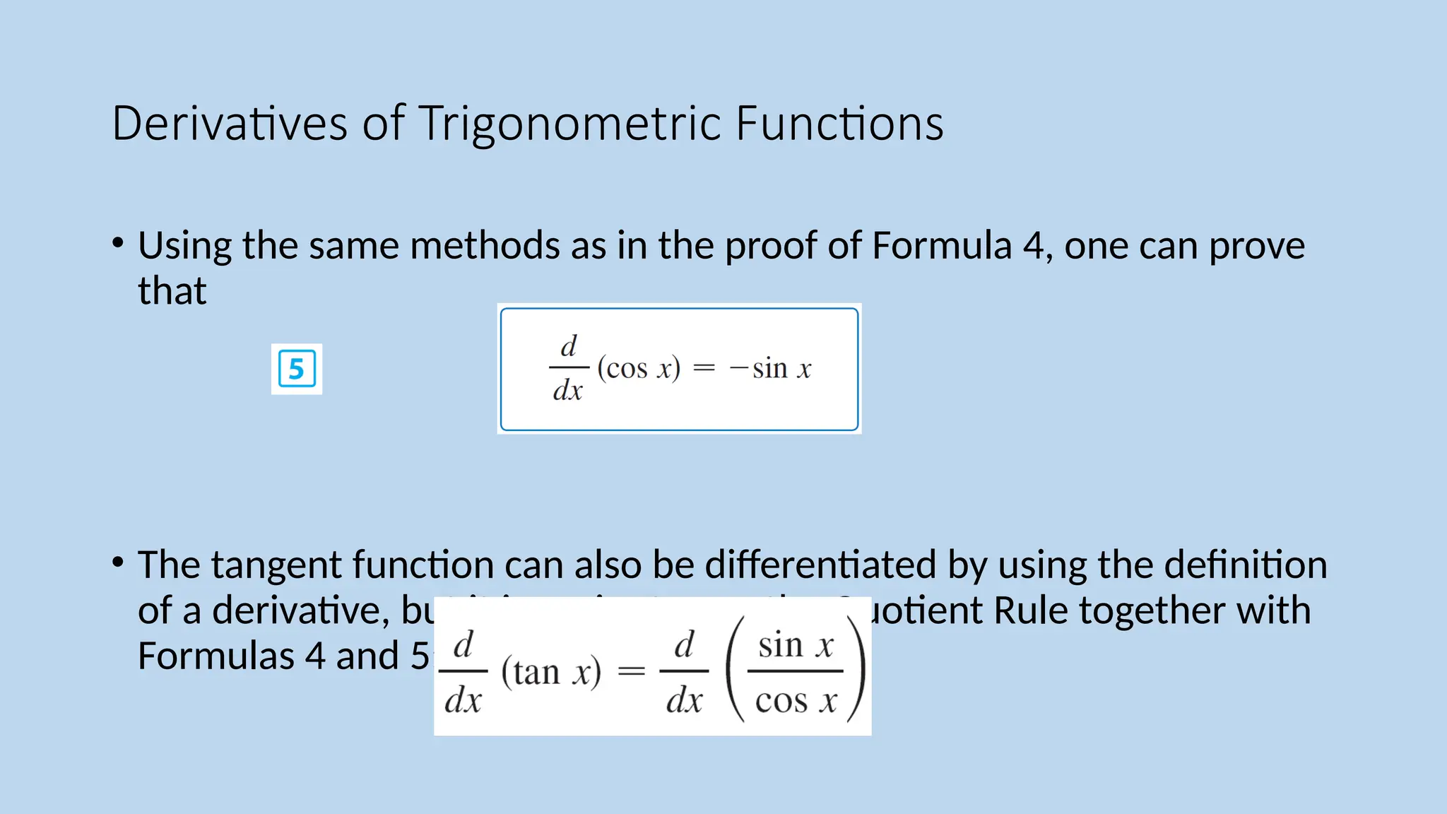
• Using the same methods as in the proof of Formula 4, one can prove
that
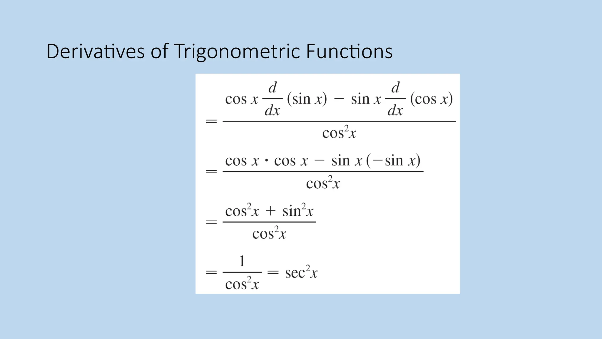
• The tangent function can also be differentiated by using the definition
of a derivative, but it is easier to use the Quotient Rule together with
Formulas 4 and 5:

61. Derivatives of Trigonometric Functions

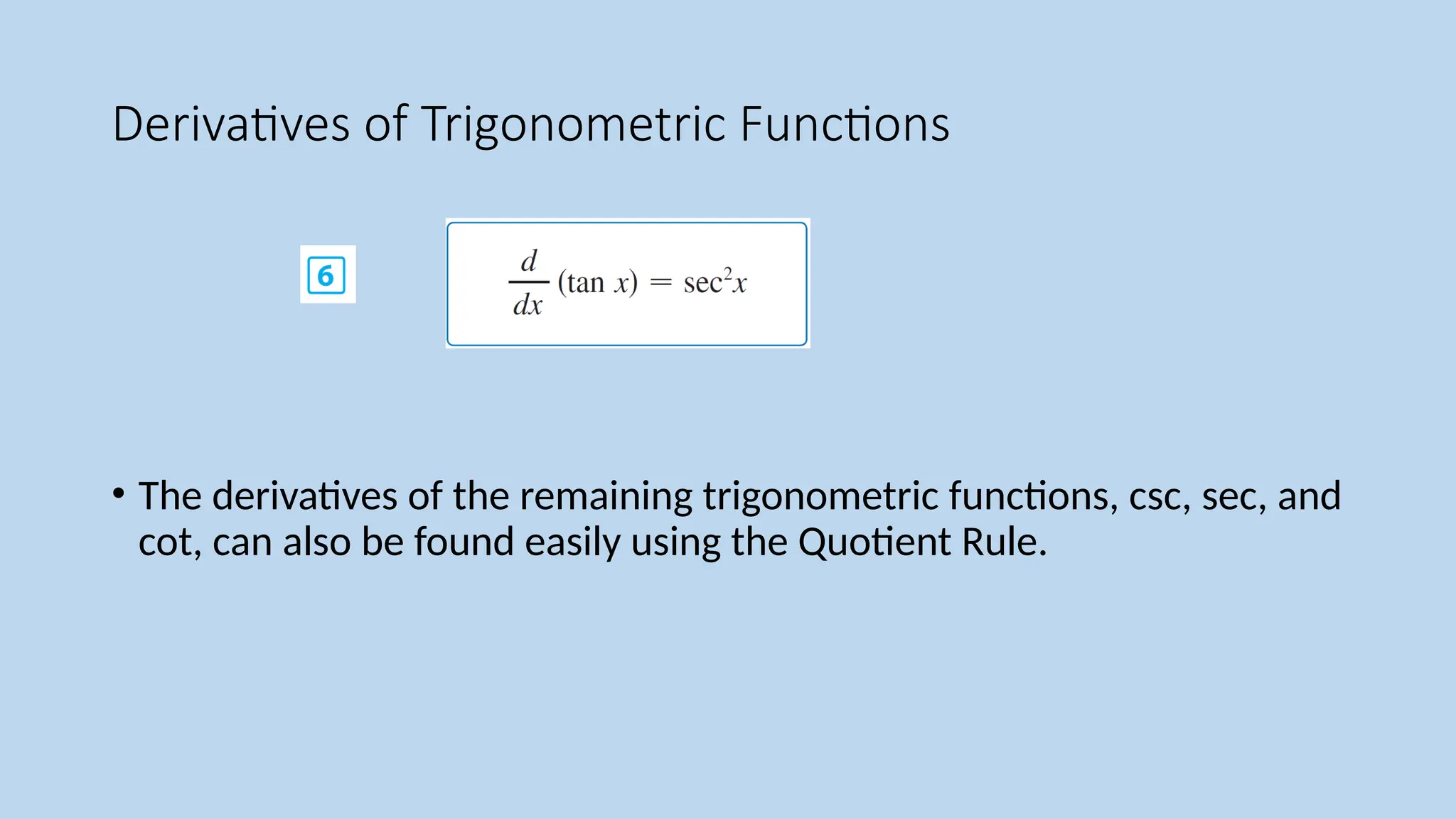
62. Derivatives of Trigonometric Functions
• The derivatives of the remaining trigonometric functions, csc, sec, and
cot, can also be found easily using the Quotient Rule.

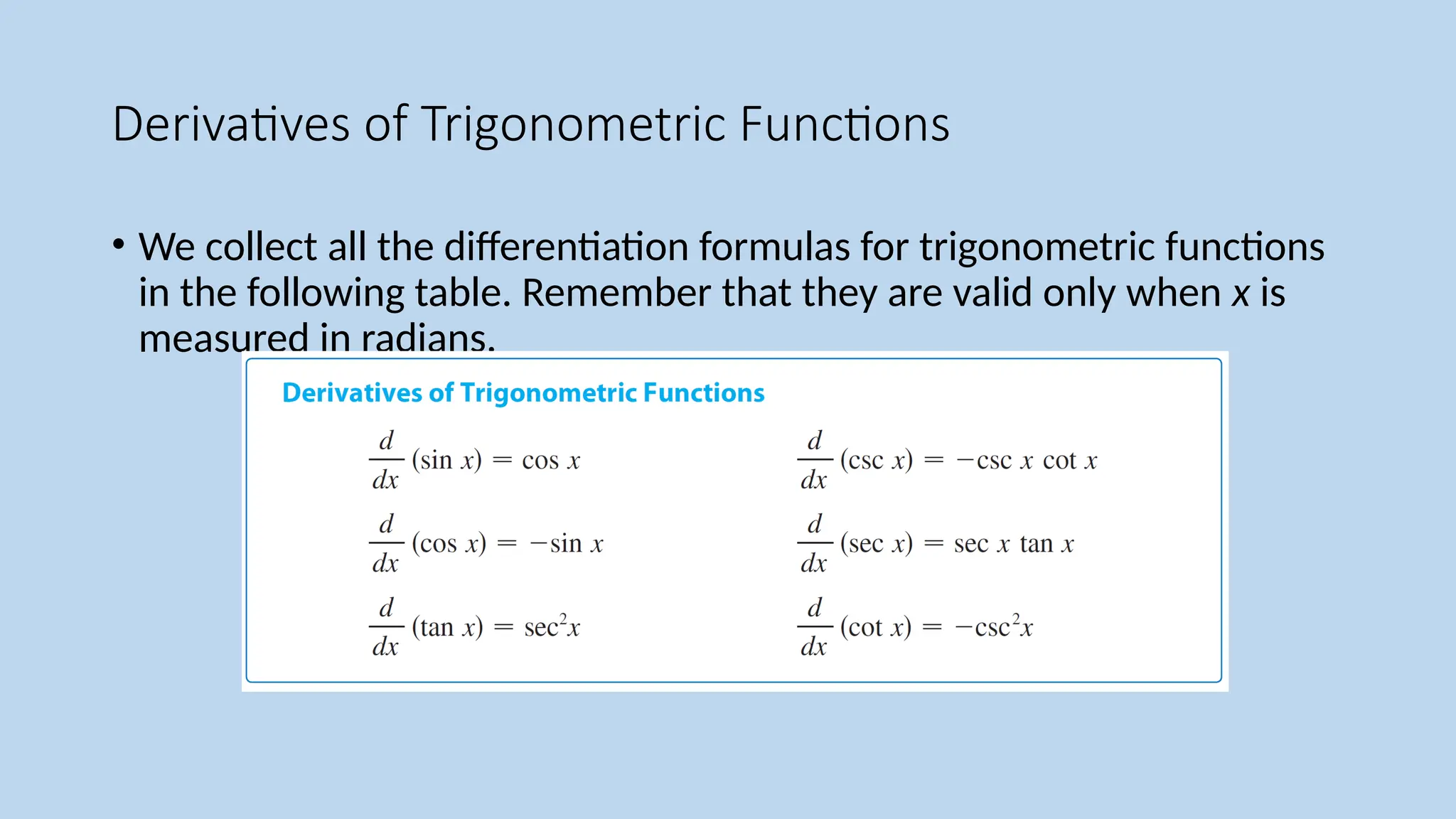
63. Derivatives of Trigonometric Functions
• We collect all the differentiation formulas for trigonometric functions
in the following table. Remember that they are valid only when x is
measured in radians.

64. Derivatives of Trigonometric Functions
• Trigonometric functions are often used in modeling
real-world phenomena. In particular, vibrations, waves, elastic
motions, and other quantities that vary in a periodic manner can be
described using trigonometric functions. In the next example we
discuss an instance of simple harmonic motion.

65. Example 3
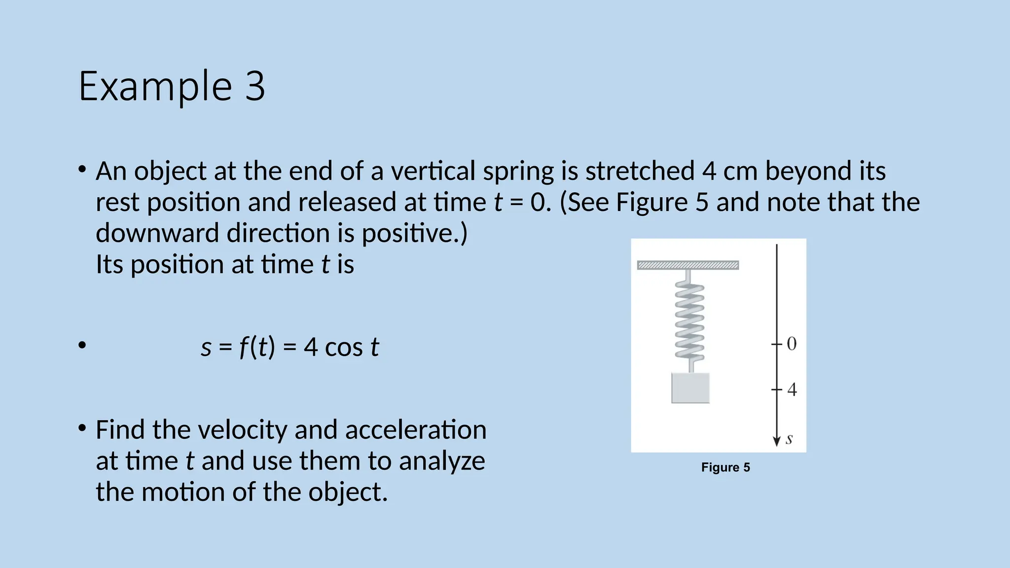
• An object at the end of a vertical spring is stretched 4 cm beyond its
rest position and released at time t = 0. (See Figure 5 and note that the
downward direction is positive.)
Its position at time t is
• s = f(t) = 4 cos t
• Find the velocity and acceleration
at time t and use them to analyze
the motion of the object.
Figure 5

66. Example 3 – Solution
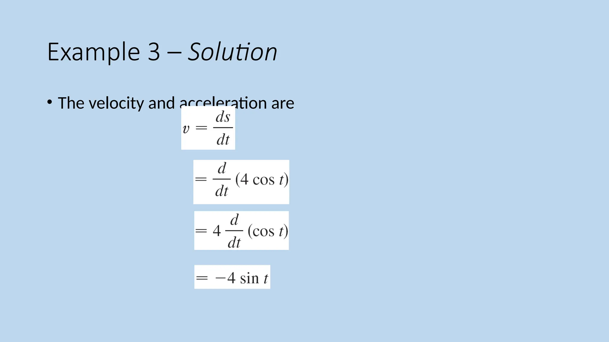
• The velocity and acceleration are

67. Example 3 – Solution
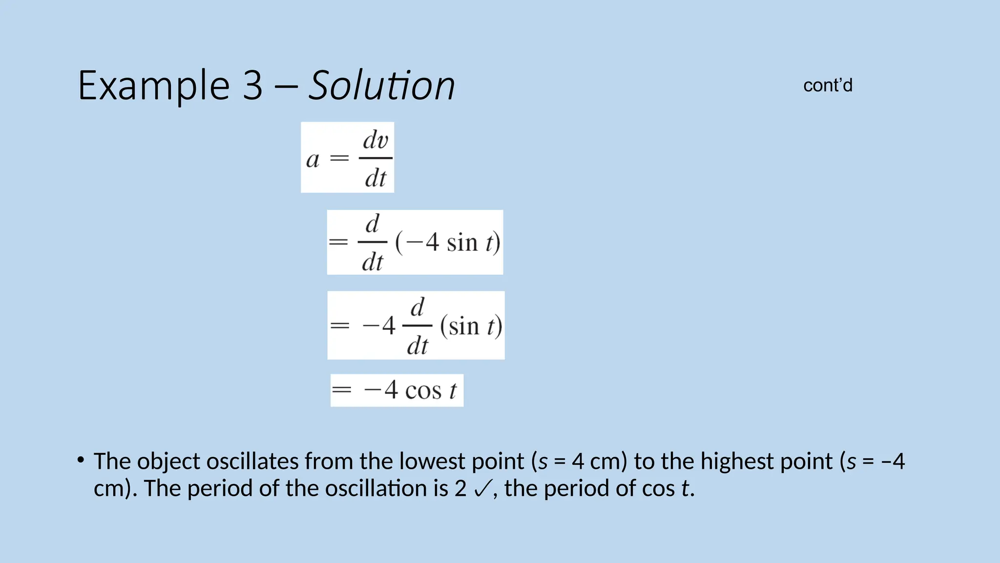
• The object oscillates from the lowest point (s = 4 cm) to the highest point (s = –4
cm). The period of the oscillation is 2, the period of cos t.
cont’d

68. Example 3 – Solution
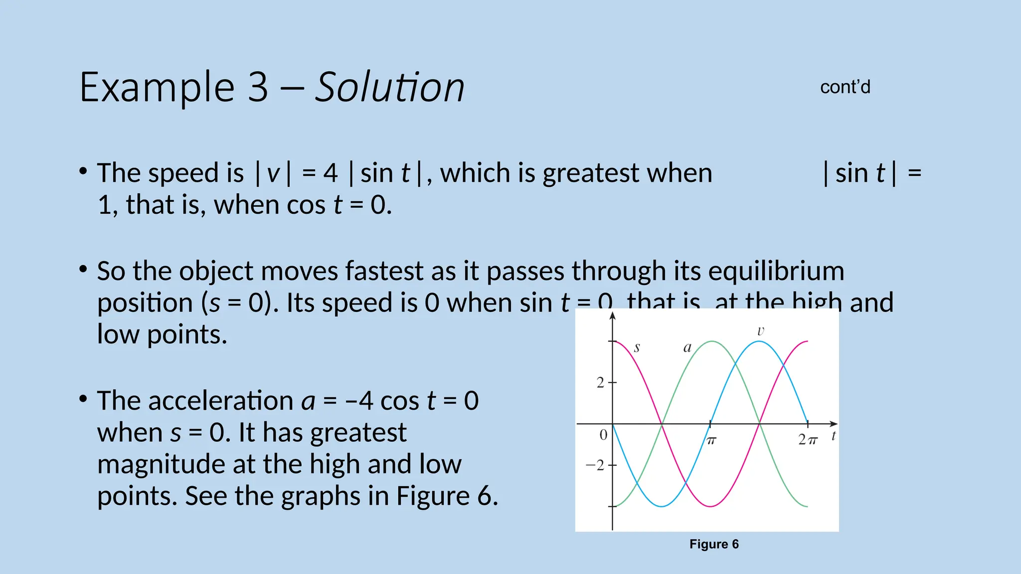
• The speed is |v| = 4 |sin t|, which is greatest when |sin t| =
1, that is, when cos t = 0.
• So the object moves fastest as it passes through its equilibrium
position (s = 0). Its speed is 0 when sin t = 0, that is, at the high and
low points.
• The acceleration a = –4 cos t = 0
when s = 0. It has greatest
magnitude at the high and low
points. See the graphs in Figure 6.
Figure 6
cont’d