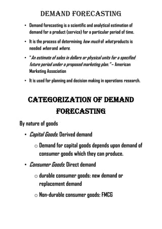
1. Demand forecasting is used to estimate future demand for products over specific time periods and is important for planning operations. 2. Demand can be categorized by the type of goods (consumer vs capital) and time period (short, medium, long term). Quantitative forecasting techniques include trend projection methods like time series analysis and regression. 3. Techniques like ARIMA combine moving averages and autoregressive methods to model trends and differences in time series data. Regression analysis uses statistical methods to model relationships between demand and influencing factors.

1. PROJECT ON: QUANTITATIVE TECHNIQUES OF
FORECASTING DEMAND

2. DEMAND FORECASTING
• Demand forecasting is a scientific and analytical estimation of
demand for a product (service) for a particular period of time.
• It is the process of determining how much of what products is
needed when and where.
• “An estimate of sales in dollars or physical units for a specified
future period under a proposed marketing plan.” – American
Marketing Association
• It is used for planning and decision making in operations research.
Categorization of Demand
Forecasting
By nature of goods
• Capital Goods: Derived demand
o Demand for capital goods depends upon demand of
consumer goods which they can produce.
• Consumer Goods: Direct demand
o durable consumer goods: new demand or
replacement demand
o Non-durable consumer goods: FMCG

3. By Time Period
• Short Term (0 to 3 months): for inventory
management and scheduling.
• Medium Term (3 months to 2 years): for production
planning, purchasing, and distribution.
• Long Term (2 years and more): may extend up to 10 to
20 years.
o For capacity planning, facility location, and
strategic planning, long term capital requirement,
and investment decisions.
HOW TO CHOOSE A DEMAND
FORECASTING TECHNIQUE
Consider the following factors affecting demand:
o Imminent objectives of forecast, whether it is for
a new product, or to gauge impact of a new
advertisement, etc.
o Cost involved, cost of forecasting should not be
more than its benefits, and here opportunity cost
of resources will also be important.

4. o Time perspective, whether the forecast is meant
for the short run or the long run
o Complexity of the technique, vis-à-vis availability
of expertise; this would determine whether the
firm would look for experts “in house” or
outsource it
o Nature and quality of available data, i.e. does the
time series show a clear trend or is it highly
unstable.
Quantitative Methods of
Demand Forecasting
Trend Projection
This statistical tool is used to predict future values of a
variable on the basis of time series data.
• Time series data are composed of:
o Secular trend (T): change occurring consistently
over a long time and is relatively smooth in its
path.
o Seasonal trend (S): seasonal variations of the
data within a year

5. o Cyclical trend (C): cyclical movement in the
demand for a product that may have a tendency to
recur in a few years
o Random events (R): have no trend of occurrence
hence they create random variation in the series.
Additive Form: Y = T + S + C + R………..(1)
Multiplicative Form: Y = T.S.C.R………….(2)
Log Y= log T + log S + log C + log R………….(3)
Methods of Trend Projection
• Graphical method
o Past values of the variable on vertical axis and
time on horizontal axis and line are plotted.
o Movement of the series is assessed and future
values of the variable are forecasted.
o simple but provides a general indication and fails
to predict future value of demand

6. Least squares method
• Based on the minimization of squared deviations
between the best fitting line and the original
observations given.
• Estimates coefficients of a linear function.
• Y=a+bX where a =intercept
• and b =slope
• The normal equations:
• ΣY=na + bΣX
• ΣXY= aΣX+ bΣX2
• Once the coefficients of the trend equation are
estimated, we can easily project the trend for future
periods.
• Solving the normal equations:
(Y Y )( X X)
A= (X X )2
Y bX

7. QUANTITATIVE METHODS
OF TREND PROJECTION
ARIMA method: also known as Box Jenkins method
• It is considered to be the most sophisticated technique
of forecasting as it combines moving average and auto
regressive techniques.
o Stage One: trend in the series is removed with
help of „differencing‟, i.e. the difference between
values at adjacent period of time.
o Stage Two: Various possible combinations are
created on basis of:
i. order of involvement of
auto regressive terms;
ii. the order of moving average terms
iii. the number of differences of the original series.
Combinations are selected which provide an adequate fit to
the series.
o Stage Three: Parameter estimation is done using
Least Squares.

8. o Stage Four: „Goodness of fit‟ is tested and if it is
not a good fit then the whole process is repeated
from Stage Two.
o Stage Five: Once a „good fit‟ is attained, its
coefficients can be used to forecast future
demand.
Quantitative Methods
• Simple (or Bivariate) Regression Analysis:
o deals with a single independent variable that
determines the value of a dependent variable.
o Demand Function: D = a+bP, where b is negative.
o If we assume there is a linear relation between D
and P, there may also be some random variation
in this relation.
Sum of Squared Errors (SSE): a measure of the predictive
accuracy
Smaller the value of SSE, the more accurate is the
regression equation.
• Nonlinear Regression Analysis
o Log linear function log D =A + B log P + e

9. where A and B are the parameters to be estimated and e
represents errors or disturbances.
Linear form of log linear function D* = a + b P* + e Where
D*= log D and P*=log P
o Multiple Regression Analysis:
D = a1+a2.P+a3.A+e
(Where A = advertising expenditure incurred).
D^ = a^1 + a^2P + a^3A, (where a1, a2 and a3 are the
parameters and e is the random error term (or
disturbance), having zero mean).
Similar to simple regression analysis, multiple regression
analysis would aim at estimation of the parameters a1, a2
and a3.
o Choose such values of the coefficients that would
minimize the sum of squares of the deviations.
Problems Associated with
Regression Analysis
• Multicollinearity: when two or more explanatory
variables in the regression model are found to be

10. highly correlated the estimated coefficients may not be
accurately determined.
• Heteroscedasticity: Classical regression models
assume that the variance of error terms is constant
for all values of the independent variables in the model;
i.e. variables are homoscedastic.
• Specification errors: Omission of one or more of the
independent variables, or when the functional form
itself is wrongly constructed or estimates a demand
function in linear form, though the function should have
been nonlinear.
• Identification problem: where the equations have
common variables, like a demand supply model.