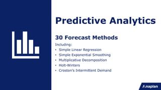
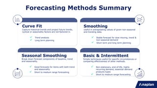
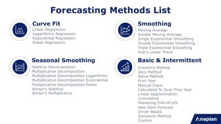
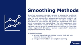
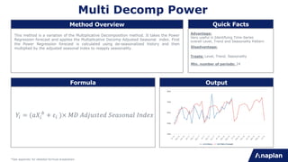
This document provides an overview of statistical forecasting methods available in Anaplan's statistical forecast model. It describes 30 different forecasting techniques, grouped into categories like curve fit methods, smoothing methods, seasonal smoothing methods, and basic/intermittent methods. Each method is briefly defined, including its formula and advantages/disadvantages. The document aims to help users understand the appropriate uses for each forecasting technique based on the characteristics of their time-series data.


![Manual Input
Advantage:
Useful for cases of new products and
promotions
Disadvantage:
There is no statistical forecasting applied
Min number of periods:
Method Overview Quick Facts
Formula Output
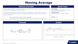
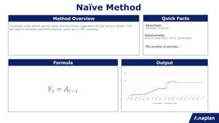
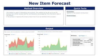
Forecasts for specific periods are entered manually by the user, based on external
factors (e.g. promotions, builds, new product introductions, etc.)
F" = [ ]](https://image.slidesharecdn.com/anaplanstatforecastingmethods-231217062707-acc3c5c6/85/Anaplan-Stat-Forecasting-Methods-pdf-31-320.jpg)


![time series.ppt [Autosaved].pdf](https://cdn.slidesharecdn.com/ss_thumbnails/timeseries-231013231623-6993e801-thumbnail.jpg?width=640&height=640&fit=bounds)


