Download as PDF, PPTX
![4 | Practical Deep Learning Examples with MATLAB
We can check the size and class of the data by typing whos in the
command window.
The MNIST images are quite small—only 28 x 28 pixels—and there are
60,000 training images in total.
The next task would be image labeling, but since the MNIST images
come with labels, we can skip that tedious step and quickly move on to
building our neural network.
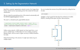
1. Accessing the Data
We begin by downloading the MNIST images into MATLAB®
. Datasets
are stored in many different file types. This data is stored as binary files,
which MATLAB can quickly use and reshape into images.
These lines of code will read an original binary file and create an array
of all the training images:
rawImgDataTrain = uint8 (fread(fid, numImg * numRows * numCols,...
'uint8'));
% Reshape the data part into a 4D array
rawImgDataTrain = reshape(rawImgDataTrain, [numRows, numCols,...
numImgs]);
imgDataTrain(:,:,1,ii) = uint8(rawImgDataTrain(:,:,ii));
>> whos imgDataTrain
Name Size Bytes Class
imgDataTrain 28x28x1x60000 47040000 uint8](https://image.slidesharecdn.com/deep-learning-practical-examples-ebook-181017091911/85/Deep-learning-practical-4-320.jpg)
![5 | Practical Deep Learning Examples with MATLAB
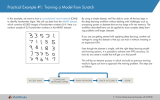
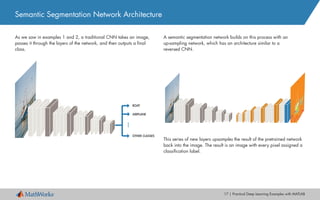
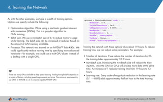
We’ll be building a CNN, the most common kind of
deep learning network.
About CNNs
A CNN passes an image through the network layers and outputs a final class. The net-
work can have tens or hundreds of layers, with each layer learning to detect different
features. Filters are applied to each training image at different resolutions, and the output
of each convolved image is used as the input to the next layer. The filters can start as very
simple features, such as brightness and edges, and increase in complexity to features that
uniquely define the object as the layers progress.
Learn More
What Is a Convolutional Neural Network? 4:44
When building a network from scratch, it’s a good idea to start with a
simple combination of commonly used layers—the lack of complexity
will make debugging much easier—but we’ll probably need to add a
few more layers to achieve the accuracy we’re aiming for.
2. Creating and Configuring Network Layers
Commonly Used Network Layers
Convolution puts the input images through a set of convolutional filters, each of which
activates certain features from the images.
Rectified linear unit (ReLU) allows for faster and more effective training by mapping nega-
tive values to zero and maintaining positive values.
Pooling simplifies the output by performing nonlinear downsampling, reducing the number
of parameters that the network needs to learn about.
Fully connected layers “flatten” the network’s 2D spatial features into a 1D vector that rep-
resents image-level features for classification purposes.
Softmax provides probabilities for each category in the dataset.
layers = [ imageInputLayer([28 28 1])
convolution2dLayer(5,20)
reluLayer
maxPooling2dLayer(2, 'Stride', 2)
fullyConnectedLayer(10)
softmaxLayer
classificationLayer() ]](https://image.slidesharecdn.com/deep-learning-practical-examples-ebook-181017091911/85/Deep-learning-practical-5-320.jpg)


![9 | Practical Deep Learning Examples with MATLAB
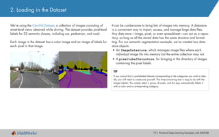
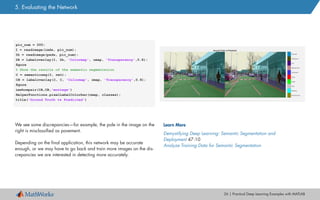
Changing the Network Configuration
Getting to 99% from 90% requires a deeper network and many rounds
of trial and error. We add more layers, including batch normalization
layers, which will help speed up the network convergence (the point at
which it responds correctly to new input).
layers = [
imageInputLayer([28 28 1])
convolution2dLayer(3,16,'Padding',1)
batchNormalizationLayer
reluLayer
maxPooling2dLayer(2,'Stride',2)
convolution2dLayer(3,32,'Padding',1)
batchNormalizationLayer
reluLayer
maxPooling2dLayer(2,'Stride',2)
convolution2dLayer(3,64,'Padding',1)
batchNormalizationLayer
reluLayer
fullyConnectedLayer(10)
softmaxLayer
classificationLayer];
The network is now “deeper.” This time, we’ll change the network but
leave the training options the same as they were before.
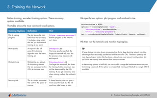
After the network has trained, we test it on 10,000 images.
This network achieves the highest accuracy of all—around 99%. We
can now use it to identify handwritten letters in online images, or even in
a live video stream.
Learn More
Training a Neural Network from Scratch with MATLAB 5:13
Deep Learning in 11 Lines of MATLAB Code 2:38
predLabelsTest = net.classify(imgDataTest);
accuracy = sum(predLabelsTest == labelsTest) / numel(labelsTest)
accuracy = 0.9880
4. Checking Network Accuracy](https://image.slidesharecdn.com/deep-learning-practical-examples-ebook-181017091911/85/Deep-learning-practical-9-320.jpg)
![11 | Practical Deep Learning Examples with MATLAB
1. Importing a Pretrained Network
We can import GoogLeNet in one line of code:
With a pretrained network, most of the heavy lifting of setting up the net-
work (selecting and organizing the layers) has already been done. This
means we can test the network on images in the categories the network
was original trained on without any reconfiguring:
TIP
Use this line of code to see all 1000 categories that GoogLeNet is trained on:
class_names = net.Layers(end).ClassNames;
Transfer Learning Tips
• Start with a highly accurate network. If a network only performs at 50% on its original
recognition task, it is unlikely to be accurate on a new recognition task.
• A model will probably be more accurate if the new recognition categories have similar
features to the original ones. For example, a network trained on dogs will probably
learn other animals relatively quickly.
% Load a pretrained network
net = googlenet;
%% Test it on an image
img = imread('peppers.png');
imgLabel = net.classify(imresize(img, [224 224]));
googlenet prediction: bell pepper](https://image.slidesharecdn.com/deep-learning-practical-examples-ebook-181017091911/85/Deep-learning-practical-11-320.jpg)
![12 | Practical Deep Learning Examples with MATLAB
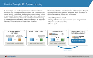
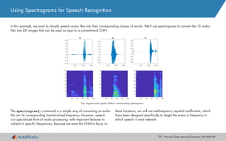
2. Configuring the Network to Perform a New Task
To train GoogLeNet to classify new images, we simply reconfigure the
last three layers of the network. These layers contain the information
needed to combine the features that the network extracts into class prob-
abilities and labels. GoogLeNet has 144 layers. Here we display the
last 5 layers of the network.
>>net.Layers(end-4:end)
We’ll reset layers 143 and 144, a softmax layer and a classification
output layer. These layers are responsible for assigning the correct cat-
egories to the input images. We want these layers to correspond to the
new categories, not to the ones that the original network learned. We
set the final fully connected layer to the same size as the number of
classes in the new dataset—five in this example.
TIP
To make speed of learning in the new layers faster than in the original layers, increase the
learning rate of the fully connected layer.
lgraph = removeLayers(lgraph, {'loss3-classifier', 'prob', ...
'output'});
numClasses = numel(unique(categories(trainDS.Labels)));
newLayers = [
fullyConnectedLayer(numClasses, 'Name','fc',...
'WeightLearnRateFactor',20,'BiasLearnRateFactor',20)
softmaxLayer('Name','softmax')
classificationLayer('Name','classoutput')];
lgraph = addLayers(lgraph,newLayers);
140 'pool5-7x7_sl' Average Pooling
141 'pool5-drop_7x7_sl' Dropout
142 'loss3-classifier' Fully Connected
143 'prob' Softmax
144 'output' Classification Output](https://image.slidesharecdn.com/deep-learning-practical-examples-ebook-181017091911/85/Deep-learning-practical-12-320.jpg)

![14 | Practical Deep Learning Examples with MATLAB
4. Evaluating the Network
Now that the network is trained, it is time to see how well it performs
on the new data.
The confusion matrix shows the network’s predictions for 150 images in
each category. If all values on the diagonal were 150, this would indi-
cate that each test image was correctly classified. Clearly, for our net-
work, this is not the case. The values outside the diagonal give a sense
of which category is getting misclassified. This can help direct us to
where we should investigate our data.
The final accuracy after training the model is 83%. While this is suffi-
cient for our example, it would not be acceptable for a real-world appli-
cation. To increase the accuracy of the model for a real-world applica-
tion, we’d continue to iterate, revisiting the training options, inspecting
the data, and reconfiguring the network.
% Classify all images from test dataset
[labels,err_test] = classify(net, testDS);
accuracy_default = sum(labels == testDS.Labels)/numel(labels);
disp(['Test accuracy is ' num2str(accuracy_default)])](https://image.slidesharecdn.com/deep-learning-practical-examples-ebook-181017091911/85/Deep-learning-practical-14-320.jpg)
![15 | Practical Deep Learning Examples with MATLAB
Even if you ultimately opt to create your own network from scratch,
transfer learning can be an excellent starting point for learning about
deep learning: You can take advantage of networks developed by ex-
perts in the field, change a few layers, and begin training—and since
the model has already learned many features from the original training
dataset, it needs less training time and fewer training images than a
model developed from scratch.
Learn More
Pretrained Convolutional Neural Networks
Transfer Learning Using GoogLeNet
Transfer Learning in 10 Lines of MATLAB Code 4:00
Transfer Learning with Neural Networks in MATLAB 4:06
4. Evaluating the Network
Finally, we visually verify the network’s performance on new images.
[label,conf] = classify(net,im);
% classify a random image
imshow(im_display);
title(sprintf('%s %.2f, actual %s', ...
char(label),max(conf),char(actualLabel))
french_fries 0.89, actual french_fries sushi 0.58, actual sushi](https://image.slidesharecdn.com/deep-learning-practical-examples-ebook-181017091911/85/Deep-learning-practical-15-320.jpg)

![21 | Practical Deep Learning Examples with MATLAB
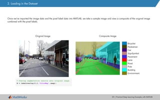
Data augmentation is a useful technique for improving the accuracy of
the trained model. In data augmentation, you increase the number of
variations in the training images by adding altered versions of the
original images. The most common types of data augmentation are
image transformations: rotation, translation, and scale.
In this example, we incorporate a random translation.
Here’s an example of a new image created by shifting the original
image 10 pixels to the left.
While the effect of this translation is subtle, it can increase the robust-
ness of the deep learning network by forcing it to learn and understand
slight variations, which are very likely to occur in a real-world system.
augmenter = imageDataAugmenter('RandXTranslation',...
[-10 10],'RandYTranslation',[-10 10]);
2. Loading in the Dataset](https://image.slidesharecdn.com/deep-learning-practical-examples-ebook-181017091911/85/Deep-learning-practical-21-320.jpg)


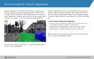
This document provides an overview of three practical deep learning examples using MATLAB: 1. Training a convolutional neural network from scratch to classify handwritten digits from the MNIST dataset, achieving over 99% accuracy after adjusting the network configuration and training options. 2. Using transfer learning to retrain the GoogLeNet model on a new food classification task with only a few categories, reconfiguring the last layers and achieving 83% accuracy on the new data. 3. An example of applying deep learning techniques for image classification to signal data classification. The examples demonstrate different approaches to training deep learning networks: training from scratch, using transfer learning, and training an existing network for a new task. All code and