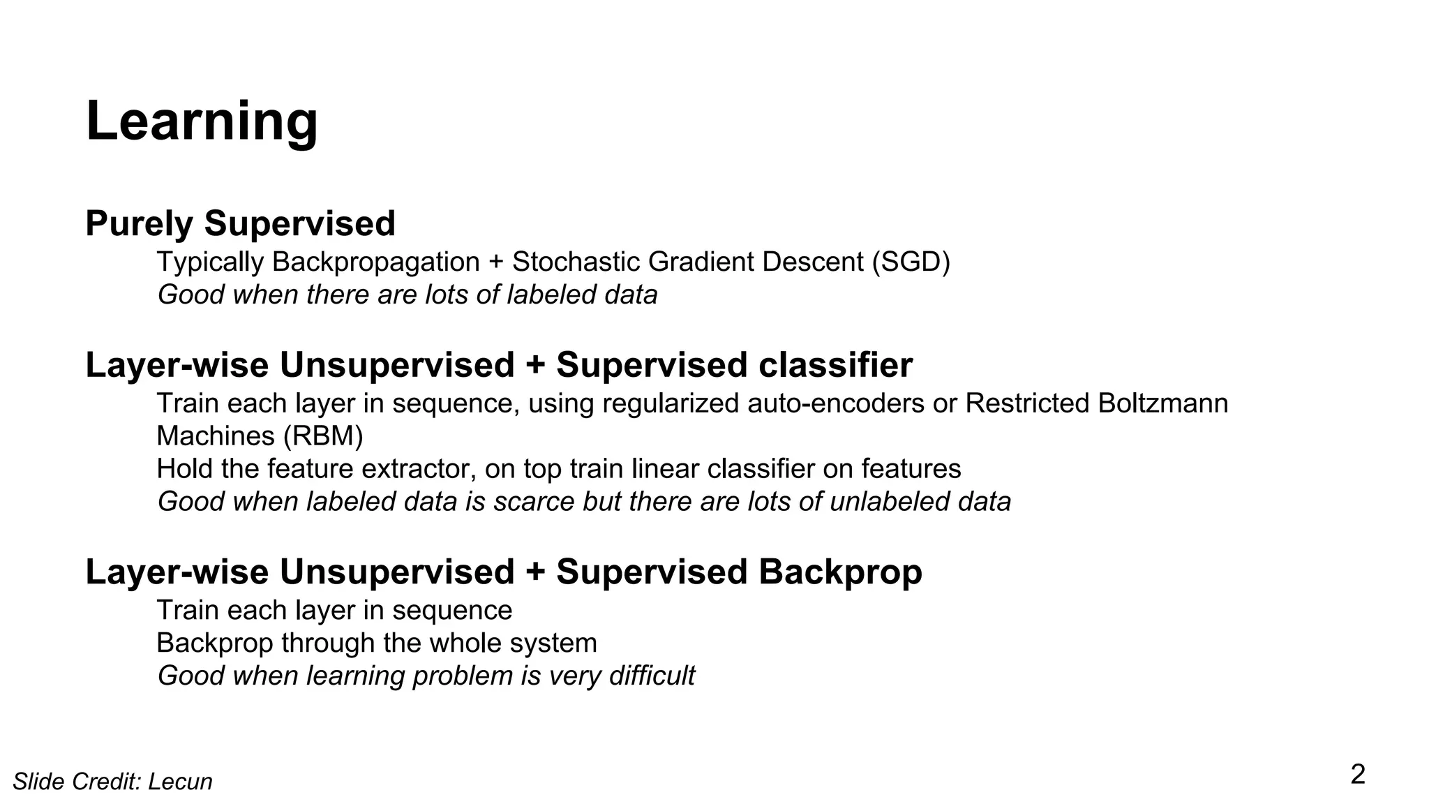
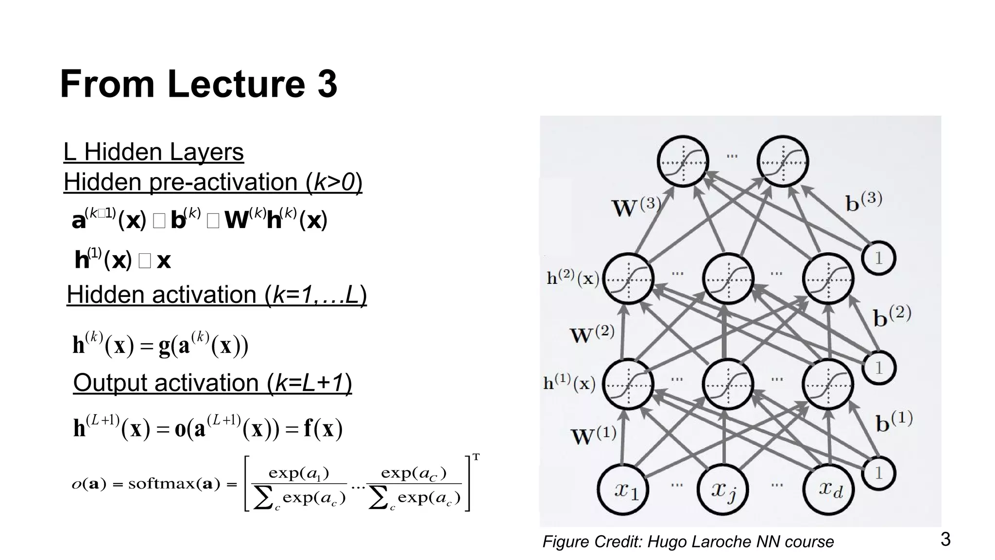
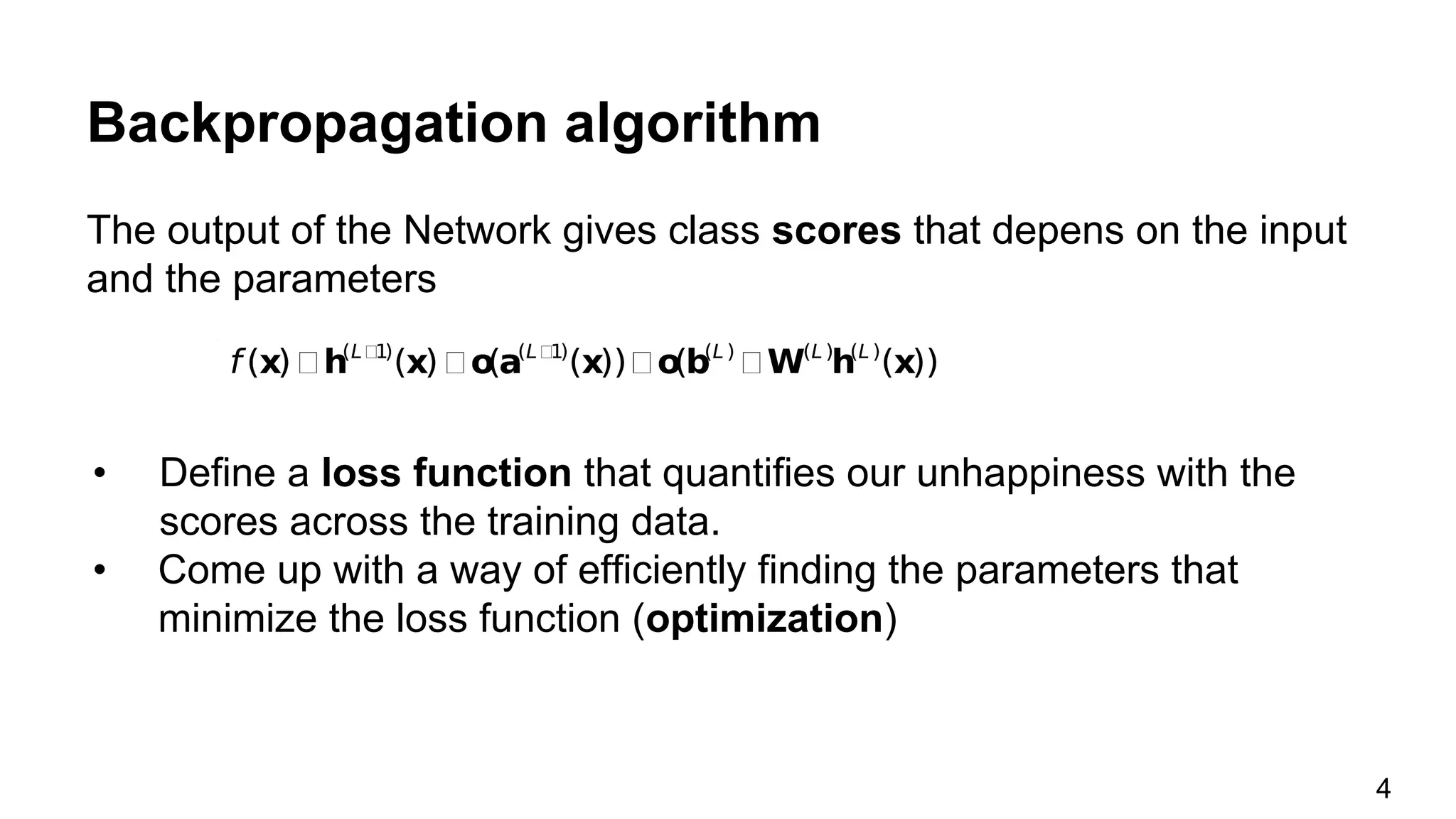
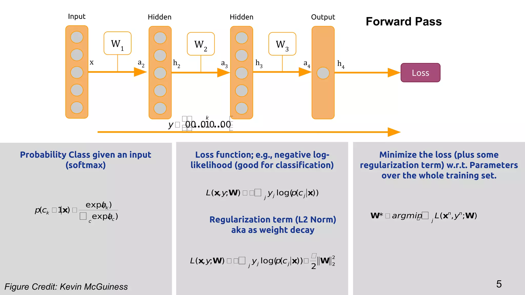
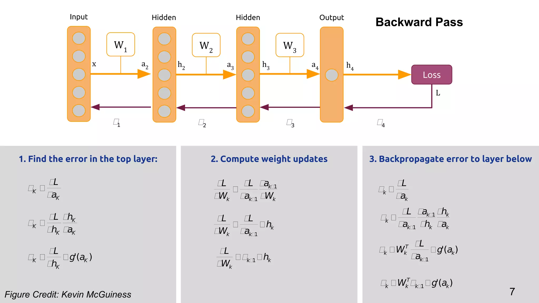
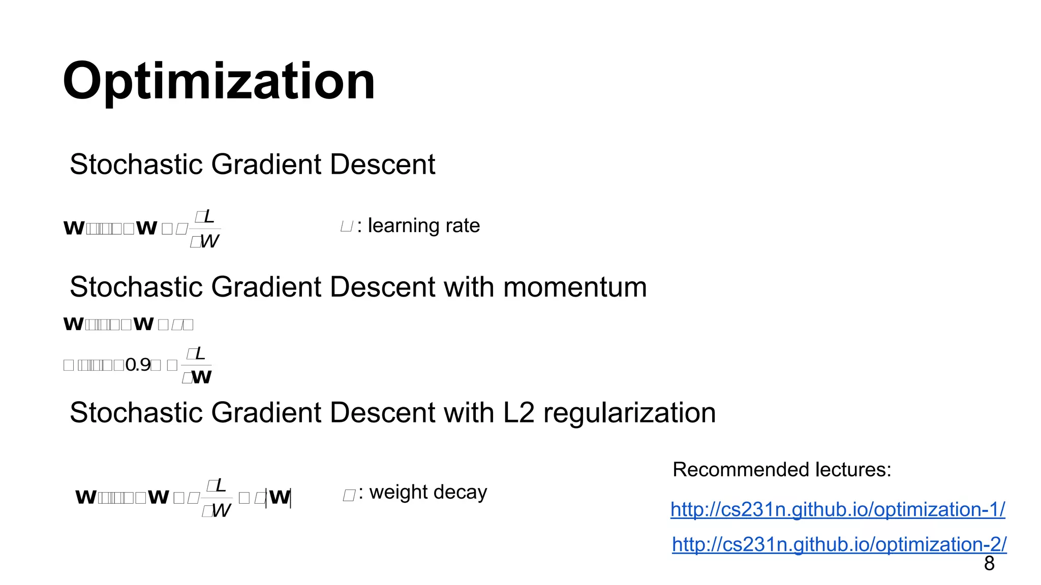
The document discusses backpropagation and optimization techniques in neural networks, emphasizing the use of supervised and unsupervised learning methods to train models effectively. It details the backpropagation algorithm's functionality, which involves minimizing a loss function using stochastic gradient descent and its variants. Additionally, it illustrates how to compute gradients iteratively through the network layers to improve parameter fitting.

1. Day 1 Lecture 4
Backward Propagation
Elisa Sayrol
[course site]

2. Learning
Purely Supervised
Typically Backpropagation + Stochastic Gradient Descent (SGD)
Good when there are lots of labeled data
Layer-wise Unsupervised + Supervised classifier
Train each layer in sequence, using regularized auto-encoders or Restricted Boltzmann
Machines (RBM)
Hold the feature extractor, on top train linear classifier on features
Good when labeled data is scarce but there are lots of unlabeled data
Layer-wise Unsupervised + Supervised Backprop
Train each layer in sequence
Backprop through the whole system
Good when learning problem is very difficult
Slide Credit: Lecun 2

3. From Lecture 3
L Hidden Layers
Hidden pre-activation (k>0)
Hidden activation (k=1,…L)
Output activation (k=L+1)
Figure Credit: Hugo Laroche NN course 3

4. Backpropagation algorithm
The output of the Network gives class scores that depens on the input
and the parameters
• Define a loss function that quantifies our unhappiness with the
scores across the training data.
• Come up with a way of efficiently finding the parameters that
minimize the loss function (optimization)
4

5. Probability Class given an input
(softmax)
Minimize the loss (plus some
regularization term) w.r.t. Parameters
over the whole training set.
Loss function; e.g., negative log-
likelihood (good for classification)
h2
h3
a3
a4 h4
Loss
Hidden Hidden Output
W2
W3
x a2
Input
W1
Regularization term (L2 Norm)
aka as weight decay
Figure Credit: Kevin McGuiness
Forward Pass
5

6. Backpropagation algorithm
• We need a way to fit the model to data: find parameters (W(k)
, b(k)
) of the
network that (locally) minimize the loss function.
• We can use stochastic gradient descent. Or better yet, mini-batch
stochastic gradient descent.
• To do this, we need to find the gradient of the loss function with respect to
all the parameters of the model (W(k)
, b(k)
)
• These can be found using the chain rule of differentiation.
• The calculations reveal that the gradient wrt. the parameters in layer k only
depends on the error from the above layer and the output from the layer
below.
• This means that the gradients for each layer can be computed iteratively,
starting at the last layer and propagating the error back through the network.
This is known as the backpropagation algorithm.
Slide Credit: Kevin McGuiness 6

7. 1. Find the error in the top layer: 3. Backpropagate error to layer below2. Compute weight updates
h2
h3
a3
a4 h4
Loss
Hidden Hidden Output
W2
W3
x a2
Input
W1
L
Figure Credit: Kevin McGuiness
Backward Pass
7

8. Optimization
Stochastic Gradient Descent
Stochastic Gradient Descent with momentum
Stochastic Gradient Descent with L2 regularization
http://cs231n.github.io/optimization-1/
http://cs231n.github.io/optimization-2/
: learning rate
: weight decay
Recommended lectures:
8