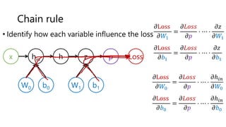
The document provides an introduction to deep learning and how to compute gradients in deep learning models. It discusses machine learning concepts like training models on data to learn patterns, supervised learning tasks like image classification, and optimization techniques like stochastic gradient descent. It then explains how to compute gradients using backpropagation in deep multi-layer neural networks, allowing models to be trained on large datasets. Key steps like the chain rule and backpropagation of errors from the final layer back through the network are outlined.


![Batch normalization
Inputs
scaled to
[0,1]
784 dim
Weights
and biases
drawn
from
N(0, 1)
R.V. with
scale
at most
784
1024 dim](https://image.slidesharecdn.com/deeplearninglecture-220919051834-9e98e995/85/DeepLearningLecture-pptx-58-320.jpg)
![Batch normalization
784 dim
Weights
and biases
drawn
from
N(0, 1)
1024 dim
𝜎1
𝜇1
𝜎2
𝜇2
𝜎3
𝜇3
𝜎𝐻
𝜇𝐻
Inputs
scaled to
[0,1]
R.V. with
scale
at most
784
R.V. with
scale
at most
784](https://image.slidesharecdn.com/deeplearninglecture-220919051834-9e98e995/85/DeepLearningLecture-pptx-59-320.jpg)
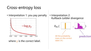
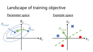
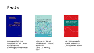
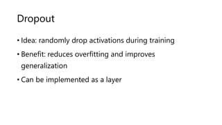
![Batch normalization [Ioffe &Szegedy, 2015]
• Idea: normalize the activation of each unit to have zero
mean and unit standard deviation using a mini-batch
estimate of mean and variance.
• Benefit: more stable and faster training. Often
generalizes better
• Can be implemented as a layer](https://image.slidesharecdn.com/deeplearninglecture-220919051834-9e98e995/85/DeepLearningLecture-pptx-60-320.jpg)

![Adaptive optimization algorithms
• Adam [Kingma & Ba 2015]: uses first and second order
statistics of the gradients so that gradients are
normalized
• Benefit: prevents the vanishing/exploding gradient
problem](https://image.slidesharecdn.com/deeplearninglecture-220919051834-9e98e995/85/DeepLearningLecture-pptx-62-320.jpg)


![[update] Introductory Parts of the Book "Dive into Deep Learning"](https://cdn.slidesharecdn.com/ss_thumbnails/d2lq1introbasicssimplemodels-190415080926-thumbnail.jpg?width=640&height=640&fit=bounds)


![[DSC Europe 25] Slobodan Dolinic - Smart and Intelligent Green Region.pptx](https://cdn.slidesharecdn.com/ss_thumbnails/0bribinjsp6ghwtvsvor-2-sigre-slobodan-dolinic-260115093812-c9c10e90-thumbnail.jpg?width=640&height=640&fit=bounds)


