1
Machine Learning: Lecture 4
Artificial Neural Networks
(Based on Chapter 4 of Mitchell T..,
Machine Learning, 1997)
2
What is an Artificial Neural
Network?
 It is a formalism for representing functions inspired from
biological systems and composed of parallel computing
units which each compute a simple function.
 Some useful computations taking place in Feedforward
Multilayer Neural Networks are:

Summation

Multiplication

Threshold (e.g., 1/(1+e ) [the sigmoidal threshold
function]. Other functions are also possible
-x
3
Biological Motivation
• Biological Learning Systems are built of very
complex webs of interconnected neurons.
• Information-Processing abilities of biological
neural systems must follow from highly parallel
processes operating on representations that are
distributed over many neurons
•ANNs attempt to capture this mode of computation
4
Multilayer Neural Network
Representation
Examples:
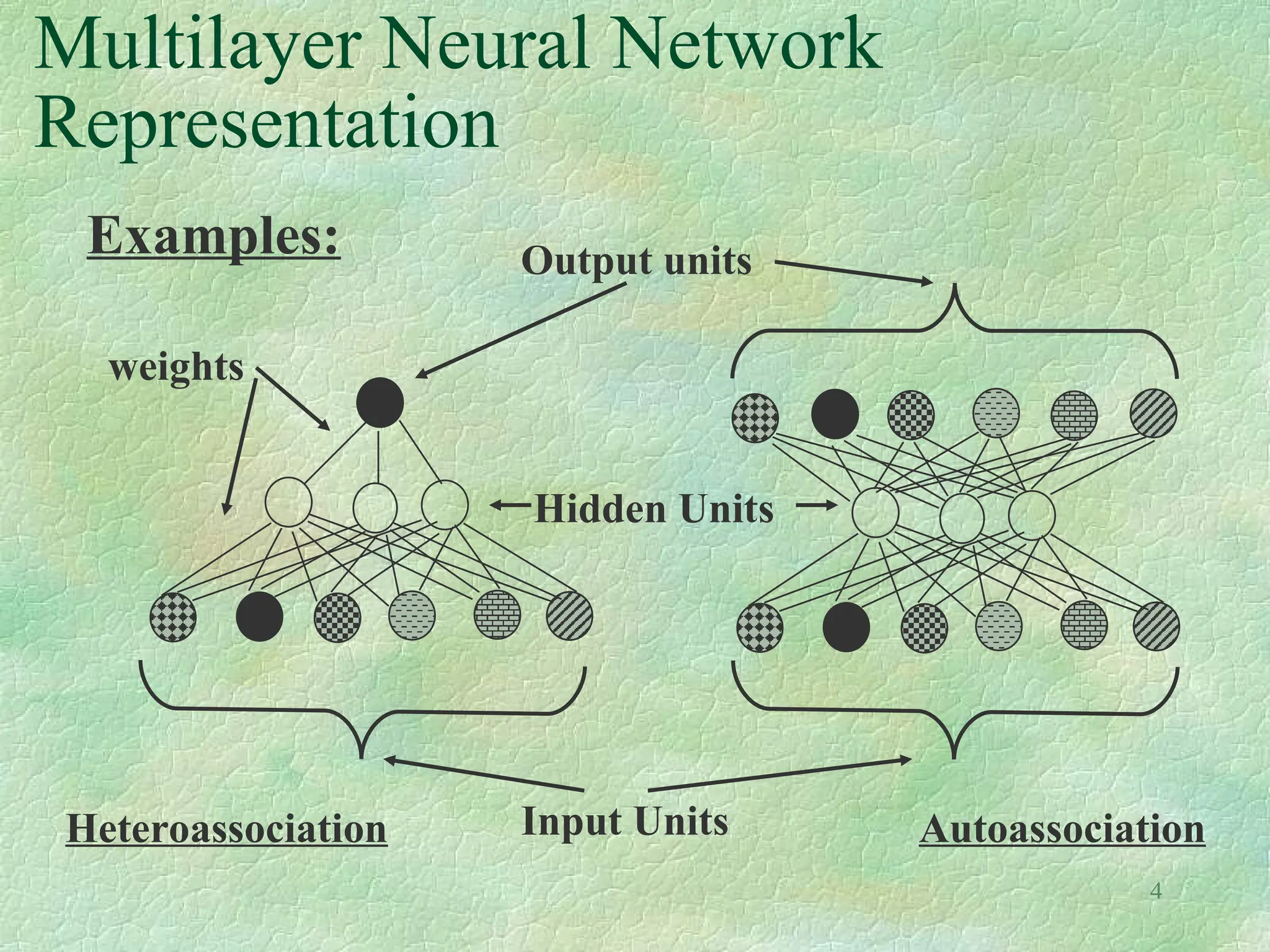
Input Units
Hidden Units
Output units
weights
Autoassociation
Heteroassociation
5
How is a function computed by a
Multilayer Neural Network?
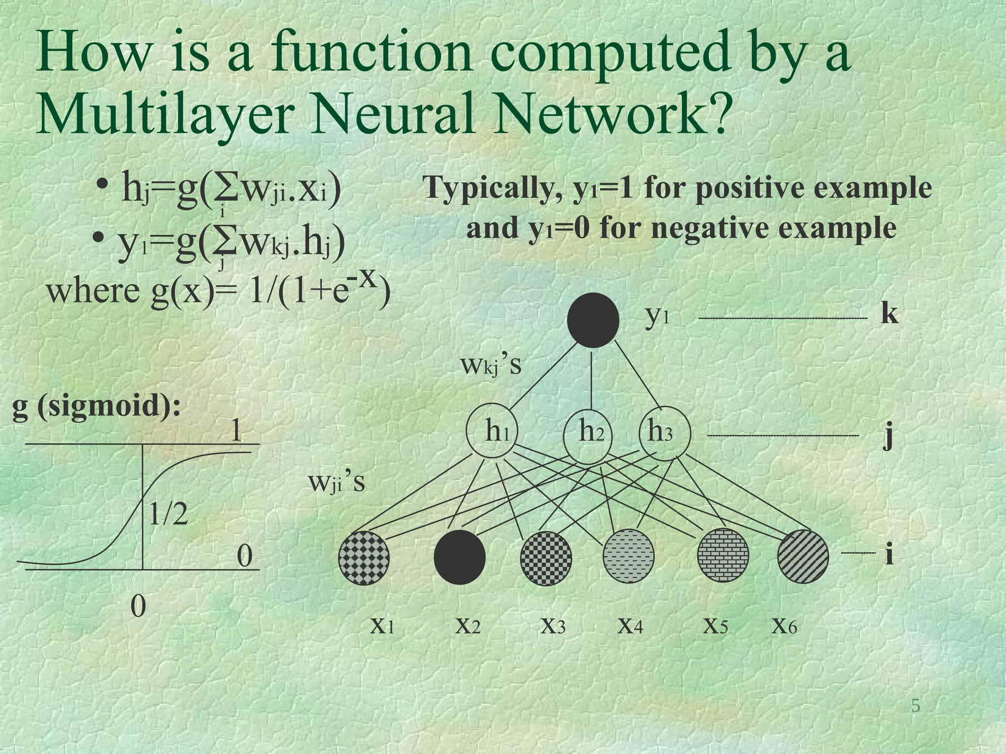
• hj=g(wji.xi)
• y1=g(wkj.hj)
where g(x)= 1/(1+e )
x1 x2 x3 x4 x5 x6
h1 h2 h3
y1 k
j
i
wji’s
wkj’s
g (sigmoid):
0
1/2
0
1
Typically, y1=1 for positive example
and y1=0 for negative example
-x
i
j
6
Learning in Multilayer Neural
Networks
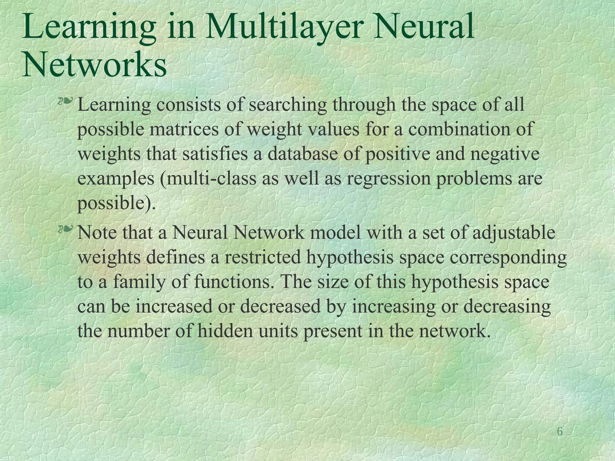
 Learning consists of searching through the space of all
possible matrices of weight values for a combination of
weights that satisfies a database of positive and negative
examples (multi-class as well as regression problems are
possible).
 Note that a Neural Network model with a set of adjustable
weights defines a restricted hypothesis space corresponding
to a family of functions. The size of this hypothesis space
can be increased or decreased by increasing or decreasing
the number of hidden units present in the network.
7
Appropriate Problems for Neural
Network Learning
 Instances are represented by many attribute-value pairs (e.g.,
the pixels of a picture. ALVINN [Mitchell, p. 84]).
 The target function output may be discrete-valued, real-valued,
or a vector of several real- or discrete-valued attributes.
 The training examples may contain errors.
 Long training times are acceptable.
 Fast evaluation of the learned target function may be required.
 The ability for humans to understand the learned target
function is not important.
8
History of Neural Networks
 1943: McCulloch and Pitts proposed a model of a neuron --> Perceptron (read
[Mitchell, section 4.4 ])
 1960s: Widrow and Hoff explored Perceptron networks (which they called
“Adelines”) and the delta rule.
 1962: Rosenblatt proved the convergence of the perceptron training rule.
 1969: Minsky and Papert showed that the Perceptron cannot deal with
nonlinearly-separable data sets---even those that represent simple function such
as X-OR.
 1970-1985: Very little research on Neural Nets
 1986: Invention of Backpropagation [Rumelhart and McClelland, but also
Parker and earlier on: Werbos] which can learn from nonlinearly-separable
data sets.
 Since 1985: A lot of research in Neural Nets!
9
Backpropagation: Purpose and
Implementation
Purpose: To compute the weights of a feedforward
multilayer neural network adaptatively, given a set
of labeled training examples.
Method: By minimizing the following cost function
(the sum of square error): E= 1/2 n=1
k=1[yk-fk(x )]
where N is the total number of training examples and K, the total
number of output units (useful for multiclass problems) and fk is the
function implemented by the neural net
N K n n 2
10
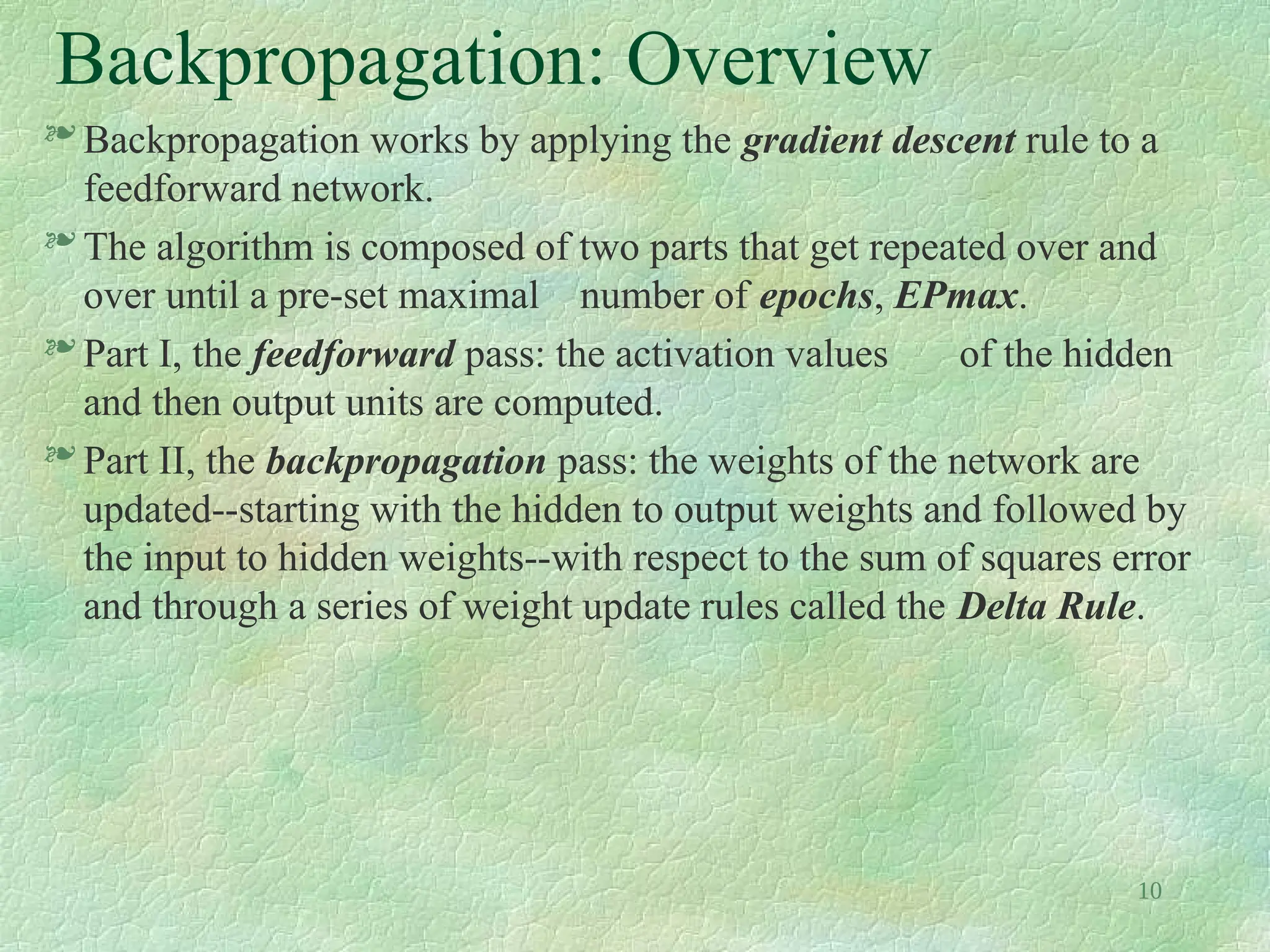
Backpropagation: Overview
 Backpropagation works by applying the gradient descent rule to a
feedforward network.
 The algorithm is composed of two parts that get repeated over and
over until a pre-set maximal number of epochs, EPmax.
 Part I, the feedforward pass: the activation values of the hidden
and then output units are computed.
 Part II, the backpropagation pass: the weights of the network are
updated--starting with the hidden to output weights and followed by
the input to hidden weights--with respect to the sum of squares error
and through a series of weight update rules called the Delta Rule.
11
Backpropagation: The Delta Rule I
For the hidden to output connections
(easy case)
wkj = - E/wkj
=  n=1[yk - fk(x )] g’(hk) Vj
=  n=1k Vj
with
N n
n
n n
n
n
N
•  corresponding to the learning rate
(an extra parameter of the neural net)
• hk = j=0 wkj Vj
•Vj = g(i=0 wjixi) and
k = g’(hk)(yk - fk(x ))
n
n
n
n n
n
n
M
d
n
M is the number of hidden units
and d the number of input units
12
Backpropagation: The Delta Rule II
For the input to hidden connections
(hard case: no pre-fixed values for the hidden units)
 wji = - E/wji
= - n=1 E/Vj Vj/wji (Chain Rule)
=  k,n[yk - fk(x )] g’(hk) wkj g’(hj)xi
=  kwkjg’(hj )xi
=  n=1j xi with
n
n
n
n
n
n
n
N
n
n
n
N n
n
• hj = i=0 wjixi
• j = g’(hj ) k=1 wkj k
• and all the other quantities already defined
d
n n
n n K n
13
Backpropagation: The Algorithm
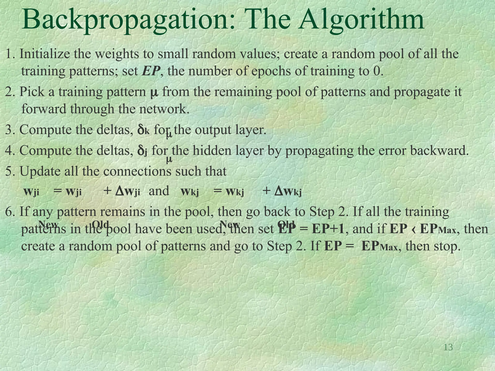
1. Initialize the weights to small random values; create a random pool of all the
training patterns; set EP, the number of epochs of training to 0.
2. Pick a training pattern  from the remaining pool of patterns and propagate it
forward through the network.
3. Compute the deltas, k for the output layer.
4. Compute the deltas, j for the hidden layer by propagating the error backward.
5. Update all the connections such that
wji = wji + wji and wkj = wkj + wkj
6. If any pattern remains in the pool, then go back to Step 2. If all the training
patterns in the pool have been used, then set EP = EP+1, and if EP  EPMax, then
create a random pool of patterns and go to Step 2. If EP = EPMax, then stop.


New Old New Old
14
Backpropagation: The Momentum
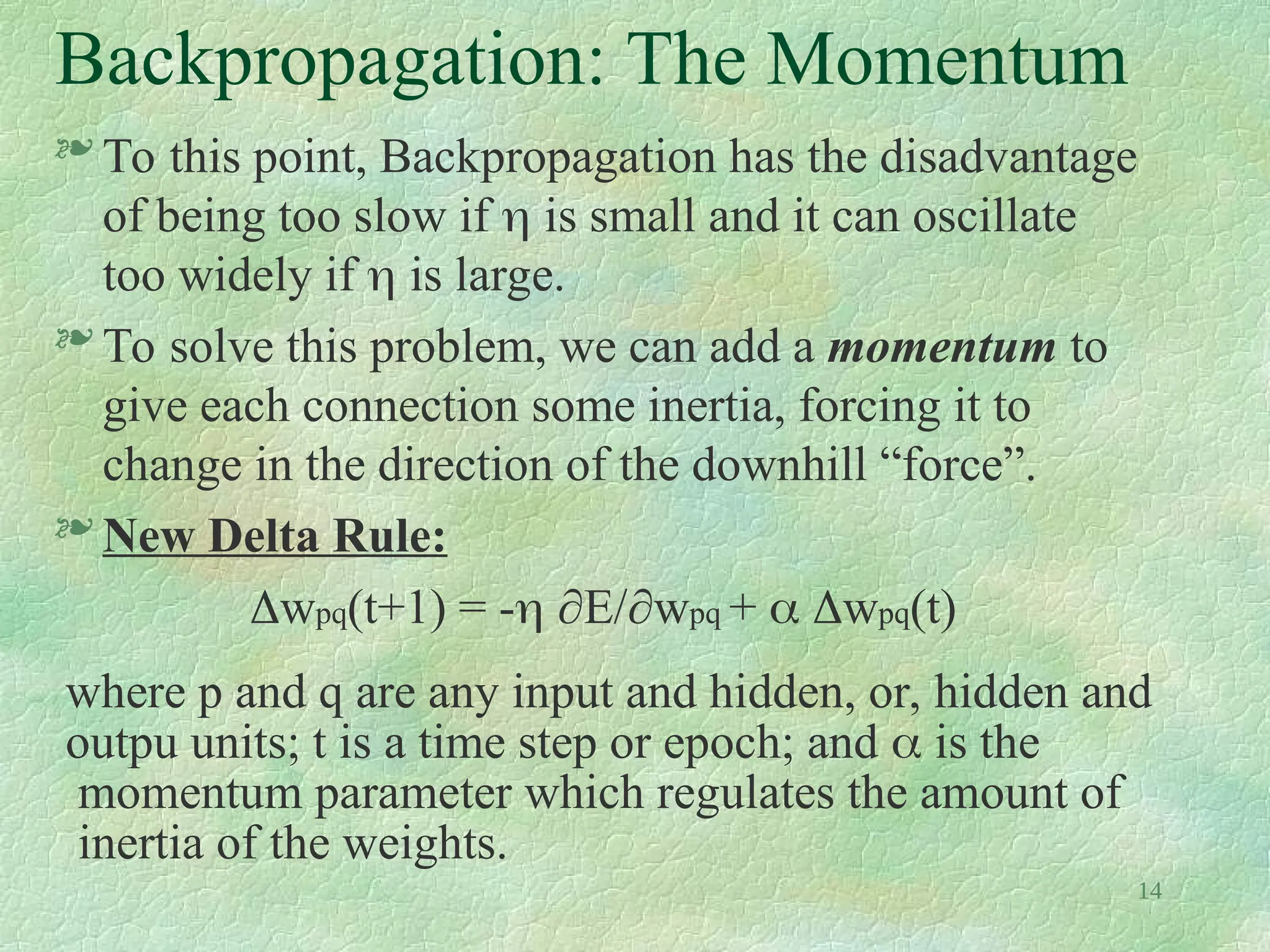
 To this point, Backpropagation has the disadvantage
of being too slow if  is small and it can oscillate
too widely if  is large.
 To solve this problem, we can add a momentum to
give each connection some inertia, forcing it to
change in the direction of the downhill “force”.
 New Delta Rule:
wpq(t+1) = - E/wpq +  wpq(t)
where p and q are any input and hidden, or, hidden and
outpu units; t is a time step or epoch; and  is the
momentum parameter which regulates the amount of
inertia of the weights.

this is a Ai topic neural network ML_Lecture_4.ppt

  • 1.
    1 Machine Learning: Lecture4 Artificial Neural Networks (Based on Chapter 4 of Mitchell T.., Machine Learning, 1997)
  • 2.
    2 What is anArtificial Neural Network?  It is a formalism for representing functions inspired from biological systems and composed of parallel computing units which each compute a simple function.  Some useful computations taking place in Feedforward Multilayer Neural Networks are:  Summation  Multiplication  Threshold (e.g., 1/(1+e ) [the sigmoidal threshold function]. Other functions are also possible -x
  • 3.
    3 Biological Motivation • BiologicalLearning Systems are built of very complex webs of interconnected neurons. • Information-Processing abilities of biological neural systems must follow from highly parallel processes operating on representations that are distributed over many neurons •ANNs attempt to capture this mode of computation
  • 4.
    4 Multilayer Neural Network Representation Examples: InputUnits Hidden Units Output units weights Autoassociation Heteroassociation
  • 5.
    5 How is afunction computed by a Multilayer Neural Network? • hj=g(wji.xi) • y1=g(wkj.hj) where g(x)= 1/(1+e ) x1 x2 x3 x4 x5 x6 h1 h2 h3 y1 k j i wji’s wkj’s g (sigmoid): 0 1/2 0 1 Typically, y1=1 for positive example and y1=0 for negative example -x i j
  • 6.
    6 Learning in MultilayerNeural Networks  Learning consists of searching through the space of all possible matrices of weight values for a combination of weights that satisfies a database of positive and negative examples (multi-class as well as regression problems are possible).  Note that a Neural Network model with a set of adjustable weights defines a restricted hypothesis space corresponding to a family of functions. The size of this hypothesis space can be increased or decreased by increasing or decreasing the number of hidden units present in the network.
  • 7.
    7 Appropriate Problems forNeural Network Learning  Instances are represented by many attribute-value pairs (e.g., the pixels of a picture. ALVINN [Mitchell, p. 84]).  The target function output may be discrete-valued, real-valued, or a vector of several real- or discrete-valued attributes.  The training examples may contain errors.  Long training times are acceptable.  Fast evaluation of the learned target function may be required.  The ability for humans to understand the learned target function is not important.
  • 8.
    8 History of NeuralNetworks  1943: McCulloch and Pitts proposed a model of a neuron --> Perceptron (read [Mitchell, section 4.4 ])  1960s: Widrow and Hoff explored Perceptron networks (which they called “Adelines”) and the delta rule.  1962: Rosenblatt proved the convergence of the perceptron training rule.  1969: Minsky and Papert showed that the Perceptron cannot deal with nonlinearly-separable data sets---even those that represent simple function such as X-OR.  1970-1985: Very little research on Neural Nets  1986: Invention of Backpropagation [Rumelhart and McClelland, but also Parker and earlier on: Werbos] which can learn from nonlinearly-separable data sets.  Since 1985: A lot of research in Neural Nets!
  • 9.
    9 Backpropagation: Purpose and Implementation Purpose:To compute the weights of a feedforward multilayer neural network adaptatively, given a set of labeled training examples. Method: By minimizing the following cost function (the sum of square error): E= 1/2 n=1 k=1[yk-fk(x )] where N is the total number of training examples and K, the total number of output units (useful for multiclass problems) and fk is the function implemented by the neural net N K n n 2
  • 10.
    10 Backpropagation: Overview  Backpropagationworks by applying the gradient descent rule to a feedforward network.  The algorithm is composed of two parts that get repeated over and over until a pre-set maximal number of epochs, EPmax.  Part I, the feedforward pass: the activation values of the hidden and then output units are computed.  Part II, the backpropagation pass: the weights of the network are updated--starting with the hidden to output weights and followed by the input to hidden weights--with respect to the sum of squares error and through a series of weight update rules called the Delta Rule.
  • 11.
    11 Backpropagation: The DeltaRule I For the hidden to output connections (easy case) wkj = - E/wkj =  n=1[yk - fk(x )] g’(hk) Vj =  n=1k Vj with N n n n n n n N •  corresponding to the learning rate (an extra parameter of the neural net) • hk = j=0 wkj Vj •Vj = g(i=0 wjixi) and k = g’(hk)(yk - fk(x )) n n n n n n n M d n M is the number of hidden units and d the number of input units
  • 12.
    12 Backpropagation: The DeltaRule II For the input to hidden connections (hard case: no pre-fixed values for the hidden units)  wji = - E/wji = - n=1 E/Vj Vj/wji (Chain Rule) =  k,n[yk - fk(x )] g’(hk) wkj g’(hj)xi =  kwkjg’(hj )xi =  n=1j xi with n n n n n n n N n n n N n n • hj = i=0 wjixi • j = g’(hj ) k=1 wkj k • and all the other quantities already defined d n n n n K n
  • 13.
    13 Backpropagation: The Algorithm 1.Initialize the weights to small random values; create a random pool of all the training patterns; set EP, the number of epochs of training to 0. 2. Pick a training pattern  from the remaining pool of patterns and propagate it forward through the network. 3. Compute the deltas, k for the output layer. 4. Compute the deltas, j for the hidden layer by propagating the error backward. 5. Update all the connections such that wji = wji + wji and wkj = wkj + wkj 6. If any pattern remains in the pool, then go back to Step 2. If all the training patterns in the pool have been used, then set EP = EP+1, and if EP  EPMax, then create a random pool of patterns and go to Step 2. If EP = EPMax, then stop.   New Old New Old
  • 14.
    14 Backpropagation: The Momentum To this point, Backpropagation has the disadvantage of being too slow if  is small and it can oscillate too widely if  is large.  To solve this problem, we can add a momentum to give each connection some inertia, forcing it to change in the direction of the downhill “force”.  New Delta Rule: wpq(t+1) = - E/wpq +  wpq(t) where p and q are any input and hidden, or, hidden and outpu units; t is a time step or epoch; and  is the momentum parameter which regulates the amount of inertia of the weights.