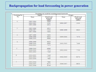
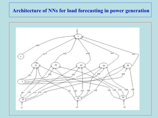
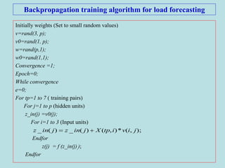
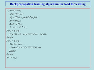
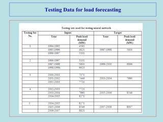
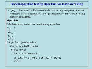
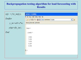
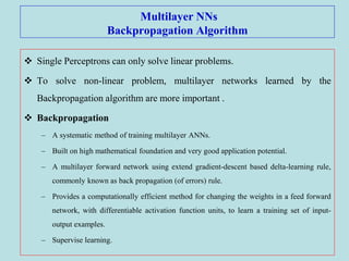
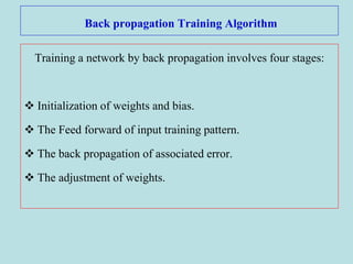
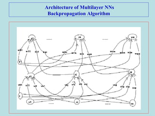
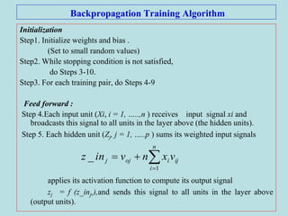
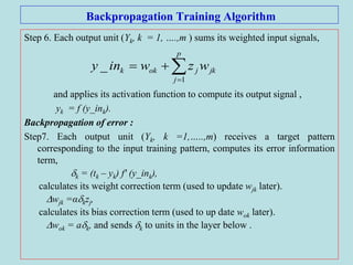
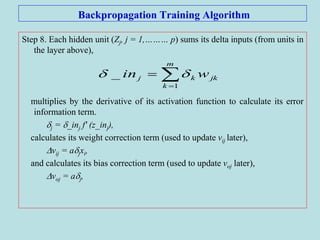
This document describes the backpropagation algorithm for training multilayer artificial neural networks (ANNs). It discusses the key aspects of the backpropagation algorithm including: the initialization of weights and biases, feedforward propagation, backpropagation of error to calculate weight updates, and updating weights and biases. It provides pseudocode for the backpropagation training algorithm and discusses factors that affect learning like learning rate and momentum. It also gives an example of using backpropagation for load forecasting in power systems, showing the network architecture, training algorithm, and results.

1. Soft Computing: Artificial Neural
Networks-Back propagation
Dr. Baljit Singh Khehra
Professor
CSE Department
Baba Banda Singh Bahadur Engineering College
Fatehgarh Sahib-140407, Punjab, India

2. Multilayer NNs
Backpropagation Algorithm
 Single Perceptrons can only solve linear problems.
 To solve non-linear problem, multilayer networks learned by the
Backpropagation algorithm are more important .
 Backpropagation
– A systematic method of training multilayer ANNs.
– Built on high mathematical foundation and very good application potential.
– A multilayer forward network using extend gradient-descent based delta-learning rule,
commonly known as back propagation (of errors) rule.
– Provides a computationally efficient method for changing the weights in a feed forward
network, with differentiable activation function units, to learn a training set of input-
output examples.
– Supervise learning.

3. Back propagation Training Algorithm
Training a network by back propagation involves four stages:
 Initialization of weights and bias.
 The Feed forward of input training pattern.
 The back propagation of associated error.
 The adjustment of weights.

4. Architecture of Multilayer NNs
Backpropagation Algorithm

5. Backpropagation Training Algorithm
Initialization
Step1. Initialize weights and bias .
(Set to small random values)
Step2. While stopping condition is not satisfied,
do Steps 3-10.
Step3. For each training pair, do Steps 4-9
Feed forward :
Step 4.Each input unit (Xi, i = 1, …..,n ) receives input signal xi and
broadcasts this signal to all units in the layer above (the hidden units).
Step 5. Each hidden unit (Zj, j = 1, …..p ) sums its weighted input signals
applies its activation function to compute its output signal
zj = f (z_inj,),and sends this signal to all units in the layer above
(output units).


n
i
ijiojj vxnvinz
1
_

6. Backpropagation Training Algorithm
Step 6. Each output unit (Yk, k = 1, ….,m ) sums its weighted input signals,
and applies its activation function to compute its output signal ,
yk = f (y_ink).
Backpropagation of error :
Step7. Each output unit (Yk, k =1,…..,m) receives a target pattern
corresponding to the input training pattern, computes its error information
term,
k = (tk – yk) f' (y_ink),
calculates its weight correction term (used to update wjk later).
wjk =αkzj,
calculates its bias correction term (used to up date wok later).
wok = ak, and sends k to units in the layer below .


p
j
jkjokk wzwiny
1
_

7. Backpropagation Training Algorithm
Step 8. Each hidden unit (Zj, j = 1,……… p) sums its delta inputs (from units in
the layer above),
multiplies by the derivative of its activation function to calculate its error
information term.
j = _inj f' (z_inj),
calculates its weight correction term (used to update vij later),
vij = ajxi,
and calculates its bias correction term (used to update voj later),
voj = aj,


m
k
jkkj win
1
_ 

8. Backpropagation Training Algorithm
Update weights and biases :
Step 9.Each output unit (Yk, k =1,……,m) updates its bias and weights
(j=0……..p) :
wjk (new) =wjk (old) + wjk,
Each hidden unit (Zj, j =1……. p) updates its bias and weights (i =
0,……,n) :
vij (new) = vij (old) + vij.
Step 10. Test stopping condition.

9. Effects of Learning rate
 Learning rate determines the size of the weight adjustments made at each
iteration and hence influences the rate of convergence.
 Poor choice of learning rate can result in a failure in convergence.
 If learning rate is too large, the search path will oscillate.
 If learning rate is too small, the descent will progress in small steps
significantly increasing the time to converge.
 Optimal selection of learning rate is necessary.

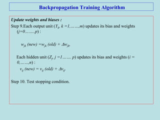
10. Momentum factor
 Momentum is a parameter that is used to improve the rate of convergance.
 If the momentum is added to the weight update formula, the convergence is
faster.
 Using momentum, the net does not proceed in the direction of the gradient,
but travels in the direction of the combination of the current gradient and
the previous direction for which the weight correction is made.
 The main purpose of momentum is to accelerate the convergence of error
propagation algorithm.
)]1()([)()1(
)]1()([)()1(


tvtvxtvtv
twtwztwtw
ijijijijij
jkjkjkjkjk



11. Backpropagation for load forecasting in power generation

12. Architecture of NNs for load forecasting in power generation

13. Backpropagation training algorithm for load forecasting
Initially weights (Set to small random values)
v=rand(3, p);
v0=rand(1, p);
w=rand(p,1);
w0=rand(1,1);
Convergence =1;
Epoch=0;
While convergence
e=0;
For tp=1 to 7 ( training pairs)
For j=1 to p (hidden units)
z_in(j) =v0(j);
For i=1 to 3 (Input units)
Endfor
z(j) = f (z_in(j),);
Endfor
);,(*),()(_)(_ jivitpXjinzjinz 

14. Backpropagation training algorithm for load forecasting
Y_in=w0+z*w;
y(tp)=f(y_in) ;
k = (T(tp) – y(tp))* f' (y_in) ;
w =α*k*z;
w0 = a*k,;
;
For j = 1 to p
;
Endfor
For j = 1 to p
For i=1 to n
;
Endfor
Endfor
v0 = aj ;
win kj *_  
))(_('*)1,(_)1,( jinzfjinj jj  
),(*)1,(*),( tpiXjajiv j

15. Backpropagation training algorithm for load forecasting
%Update weights and biases
w(new) =w (old) + w;
w0(new) =w0 (old) + w0;
v(new) =v (old) + v;
v0(new) =v0 (old) + v0;
Endfor
if e<TSE
convergence=0;
endif
Epoch=Epoch+1;
Endwhile
display (‘ Total Epoch performed’);
display (epoch);
display (‘Error’);
display (e);
display (‘Final weights &bias’);
w(new);
w0(new);
v(new);
v0(new);
    2
tpytpTee 

16. Activation functions for load Forecasting
 Performance of back propagation algorithm for load forecasting is
measured at two different activation functions:
1. Sigmoid function
Derivative of sigmoid function
2. Hyperbolic tangent function
Derivative of Hyperbolic tangent function
x
e
xf 


1
1
)(
2
'
)1(
)( x
ax
e
ae
xf 



x
x
e
e
xf 2
2
1
1
)( 




22
2
)1(
4
)(' x
x
e
e
xf 




17. Results

18. Results

19. Testing Data for load forecasting

20. Backpropagation testing algorithm for load forecasting
Let be a matrix which contains data for testing, every row of matrix
represents different testing set. In the proposed study, for testing 5 testing
pairs are considered.
Algorithm:
Calculated weights and bias from training algorithm
;
;
;
;
For tp=1 to 5 ( testing pairs)
For j=1 to p (hidden units)
Z_in(j) =v0(j);
For i=1 to 3 (Input units)
Endfor
35X
pv 3
pv 10
1pw
110 w
);,(*),()(_)(_ jivitpXjinzjinz 

21. Backpropagation testing algorithm for load forecasting with
Results
z(j) = f (z_in(j),);
Endfor
y_in=w0+z*w;
y(tp)=f(y_in) ;
End