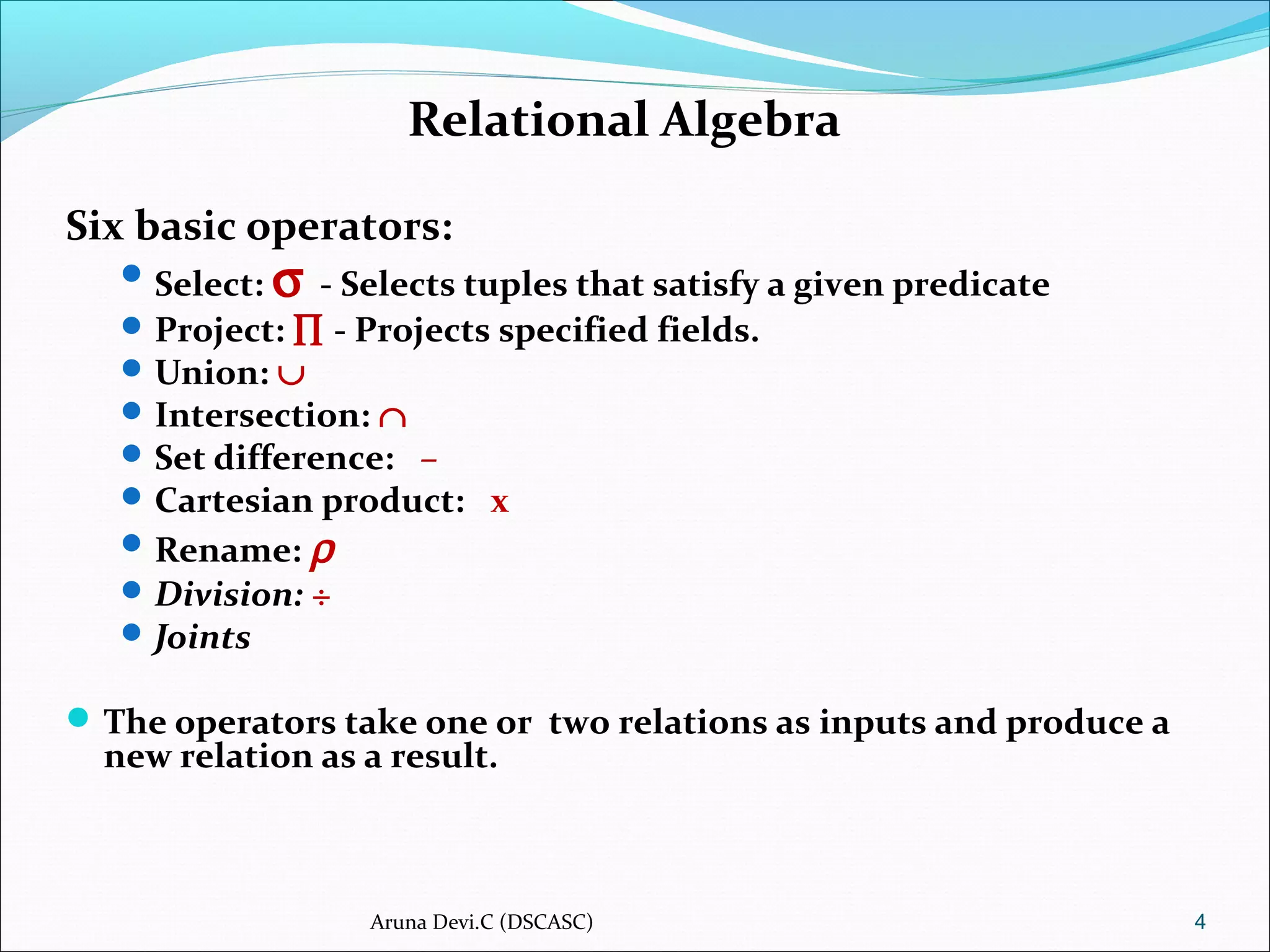
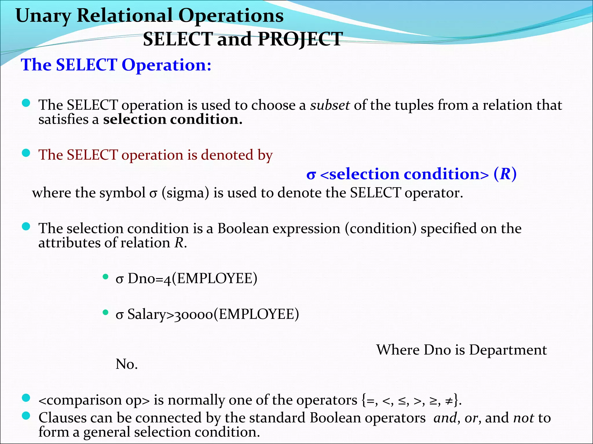
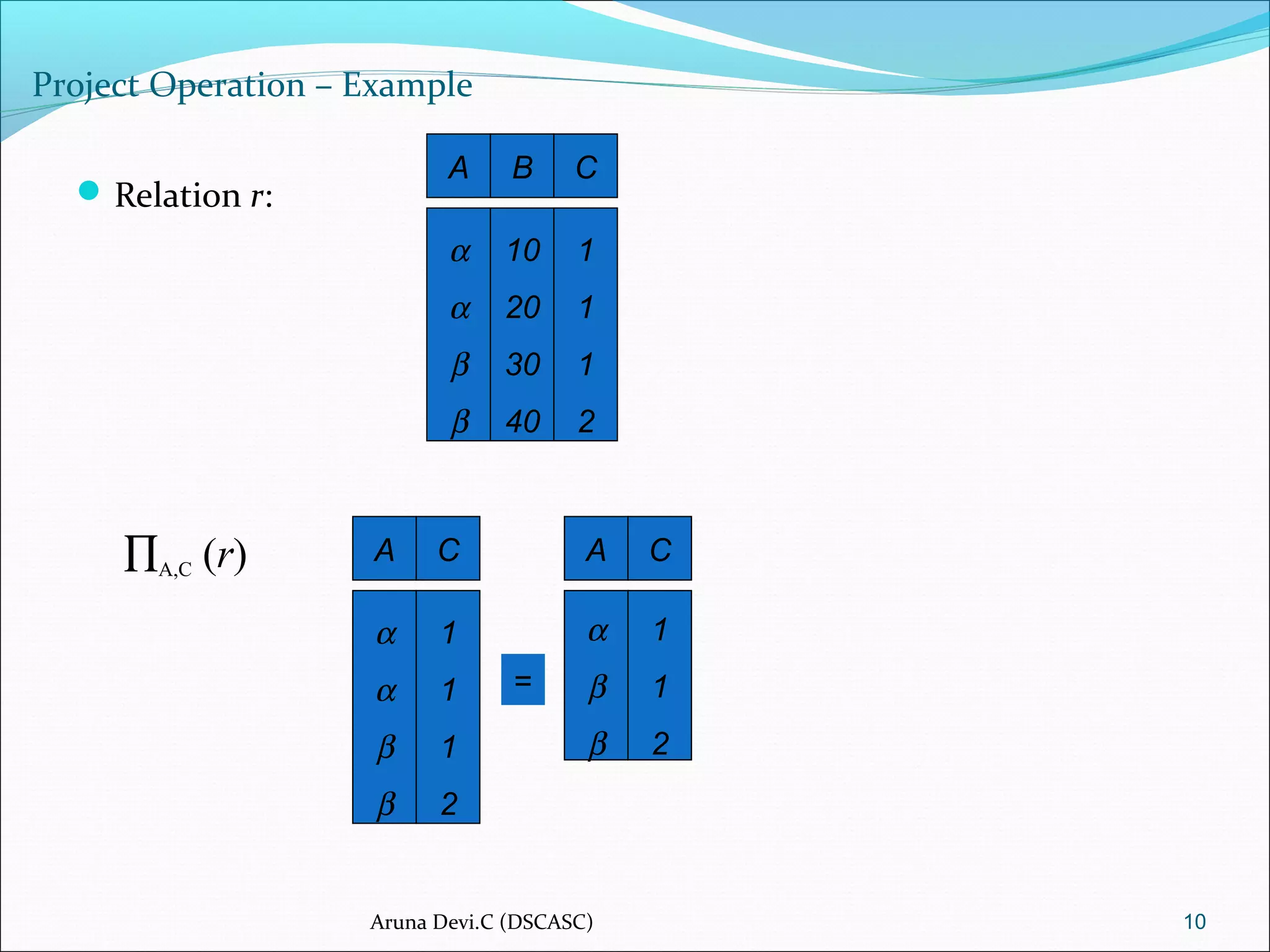
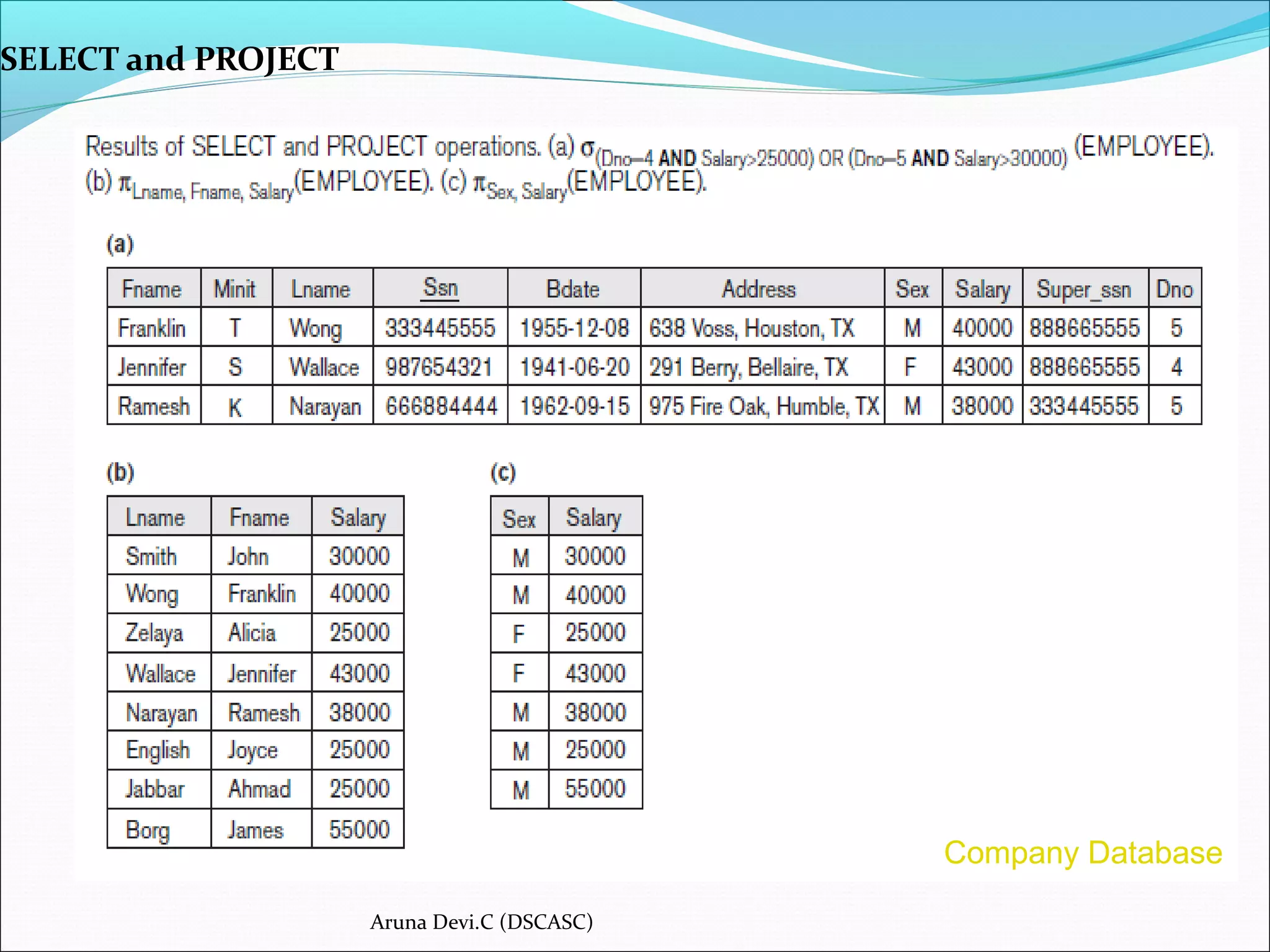
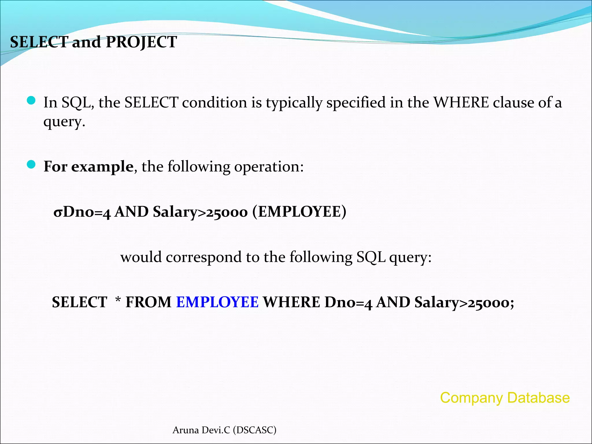
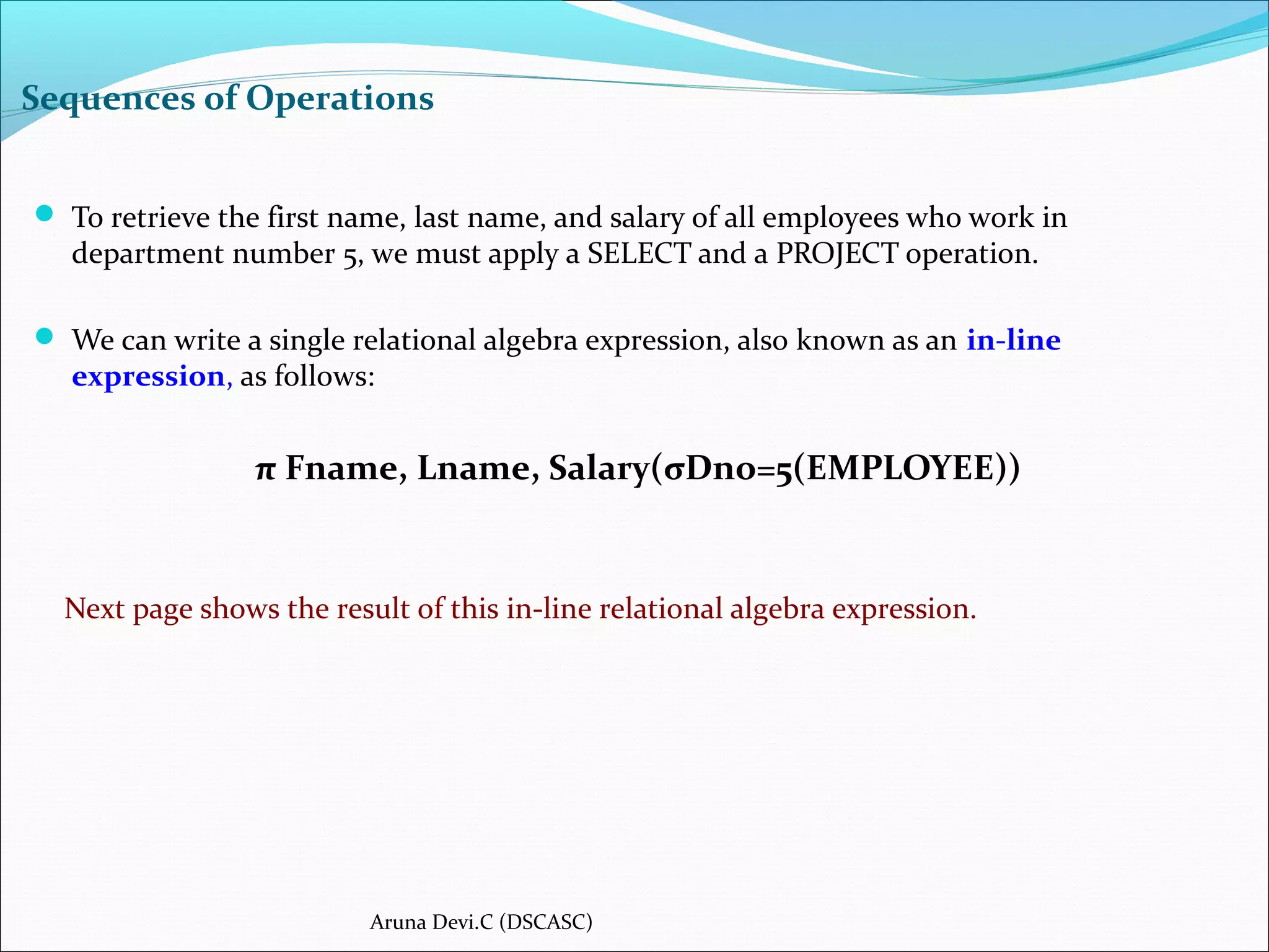
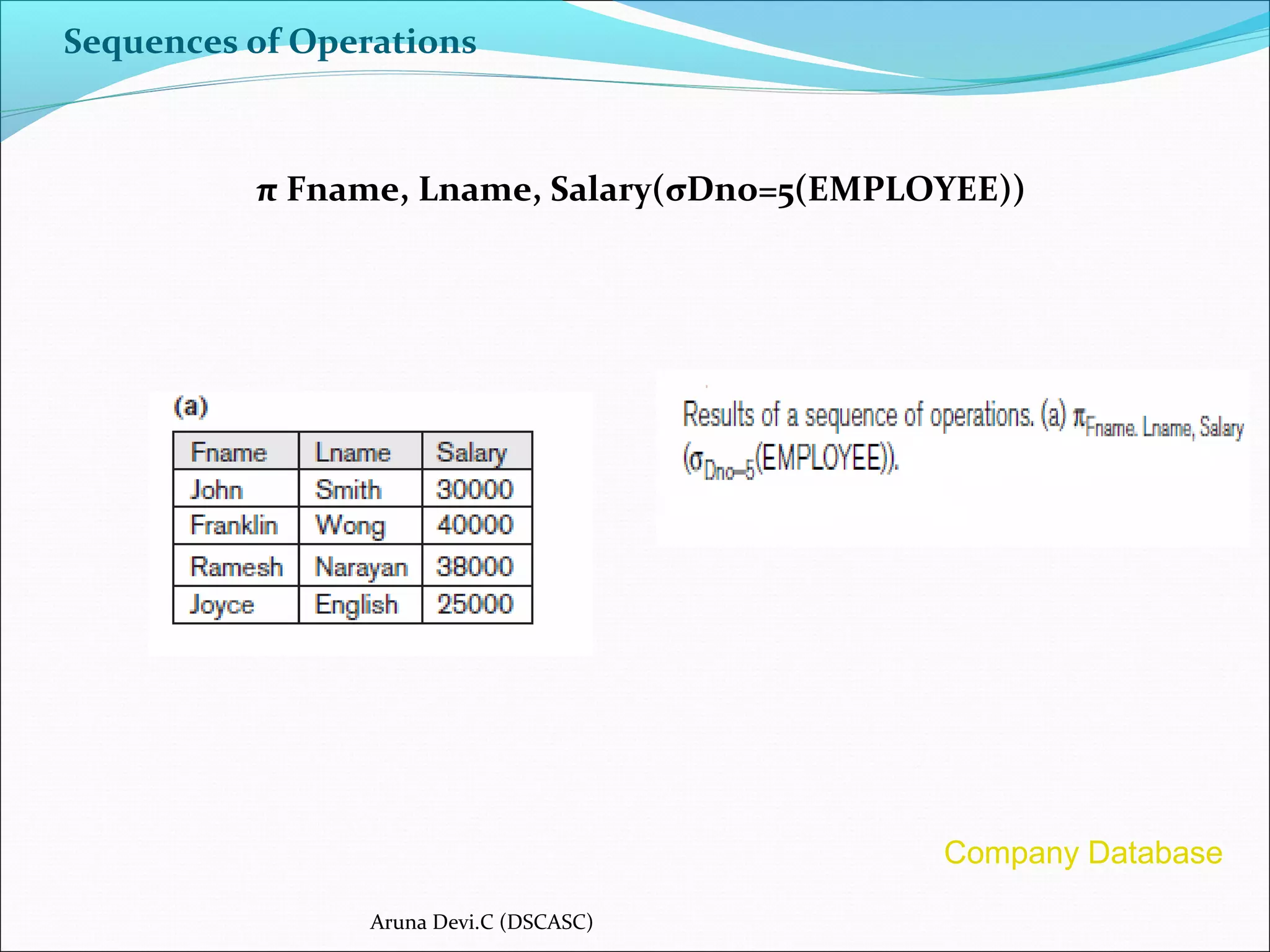
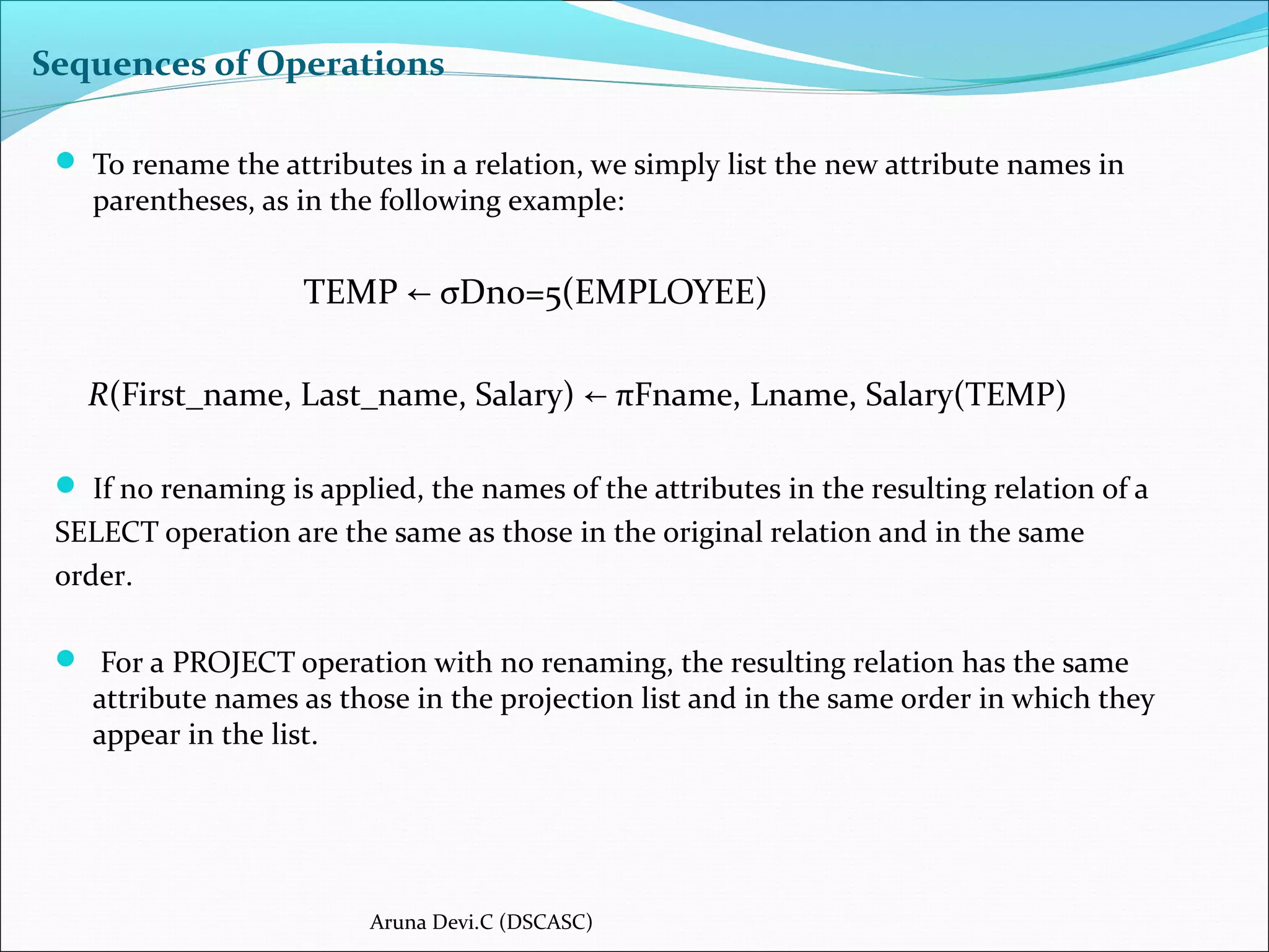
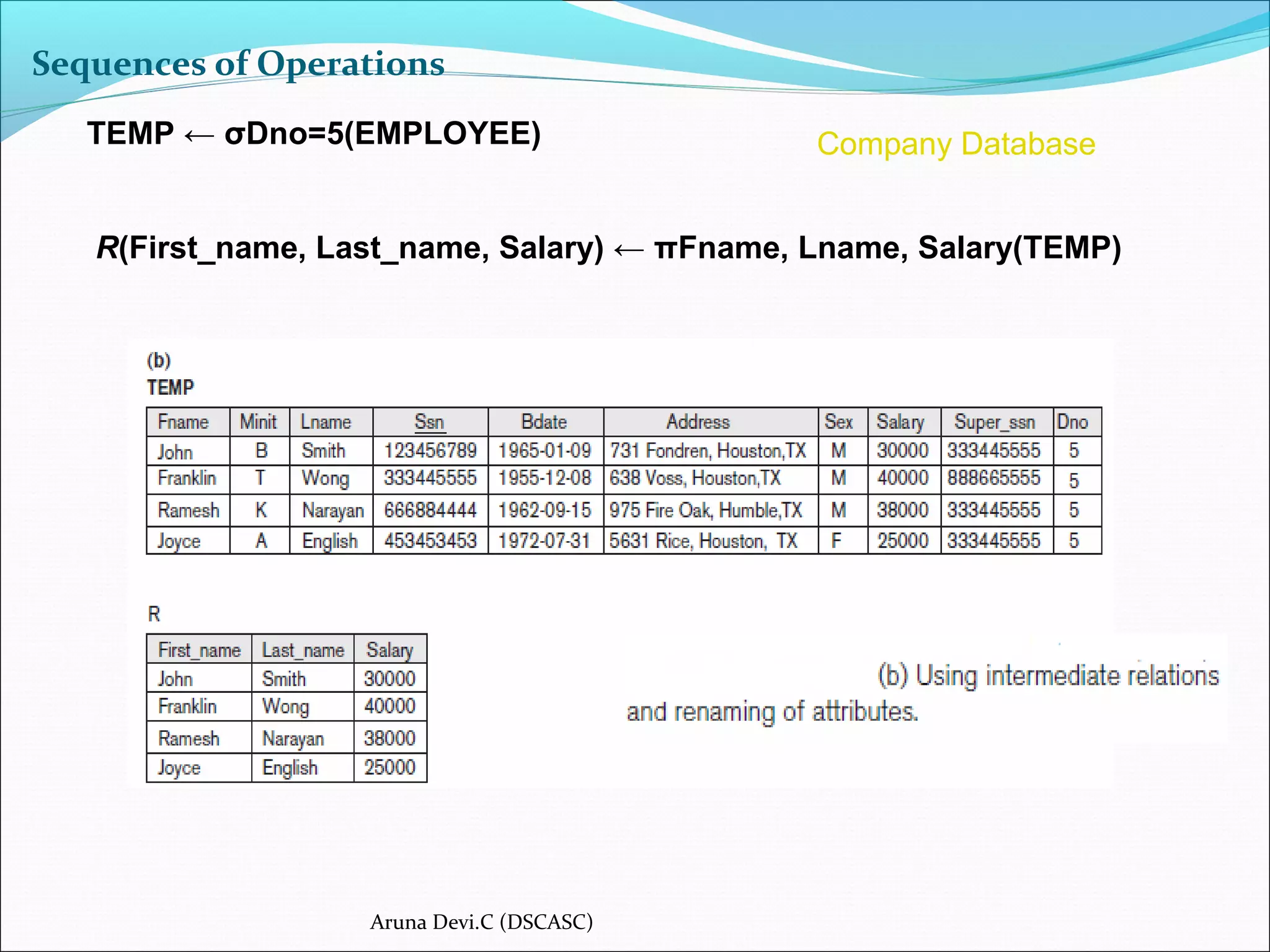
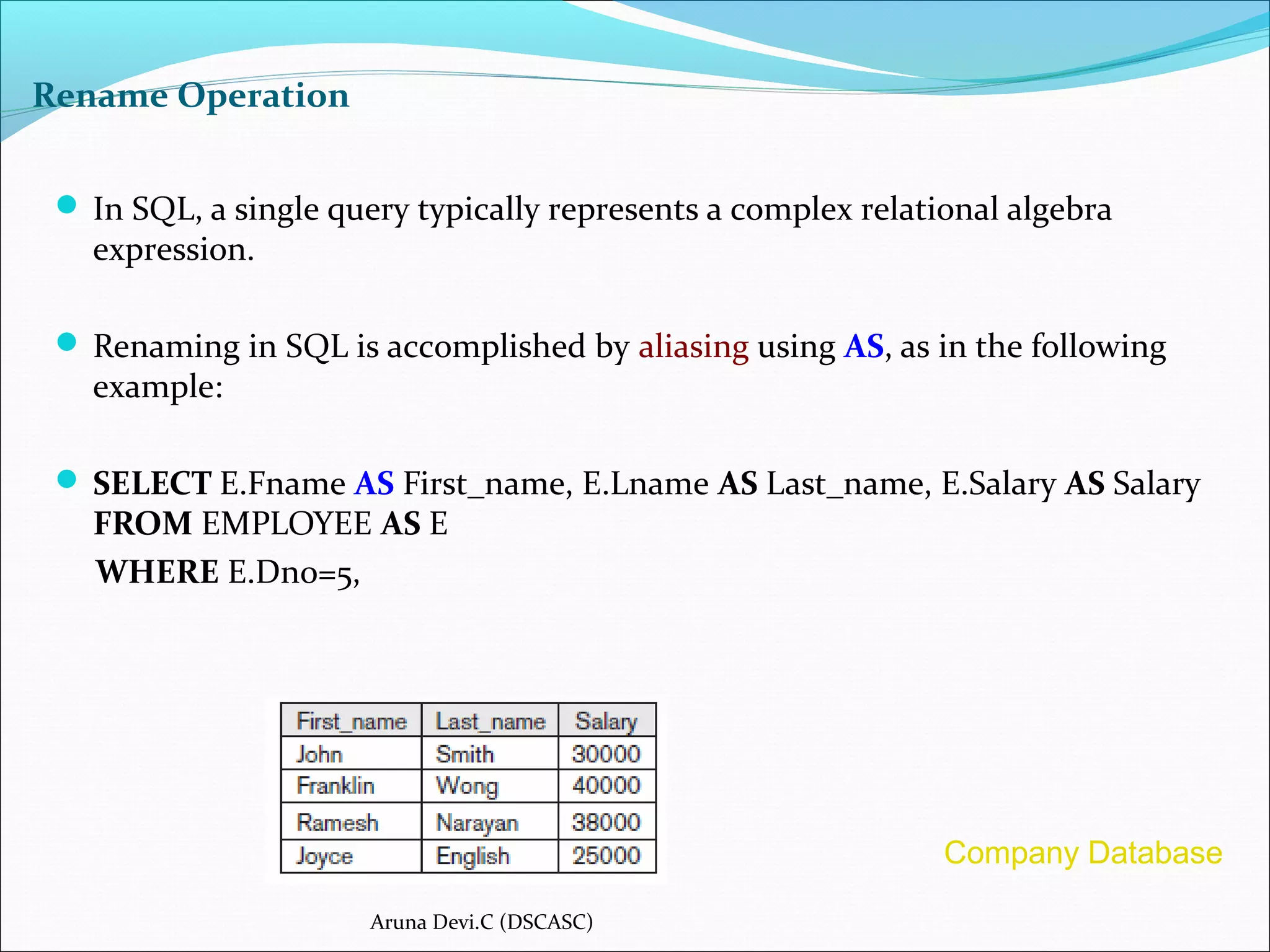
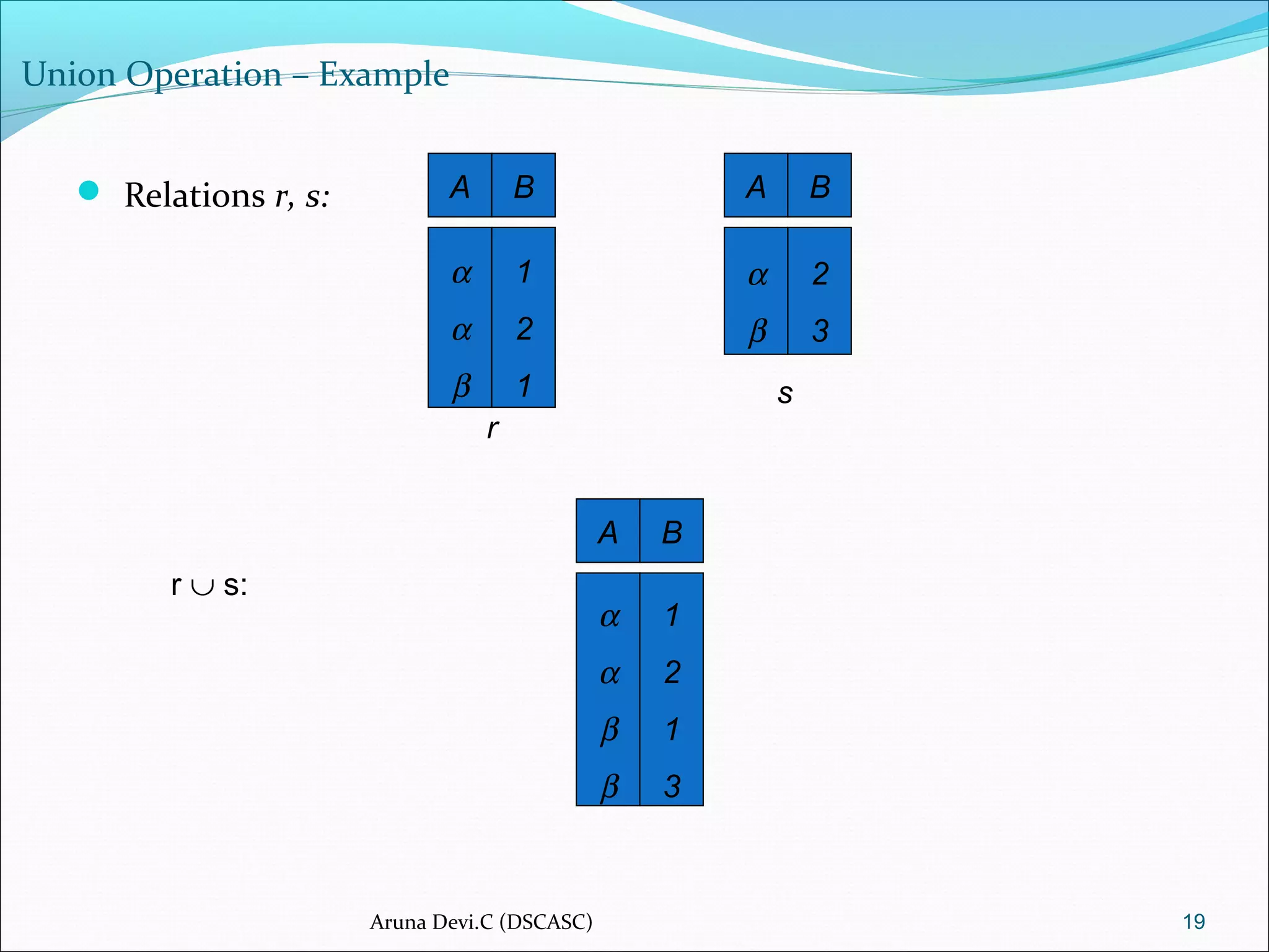
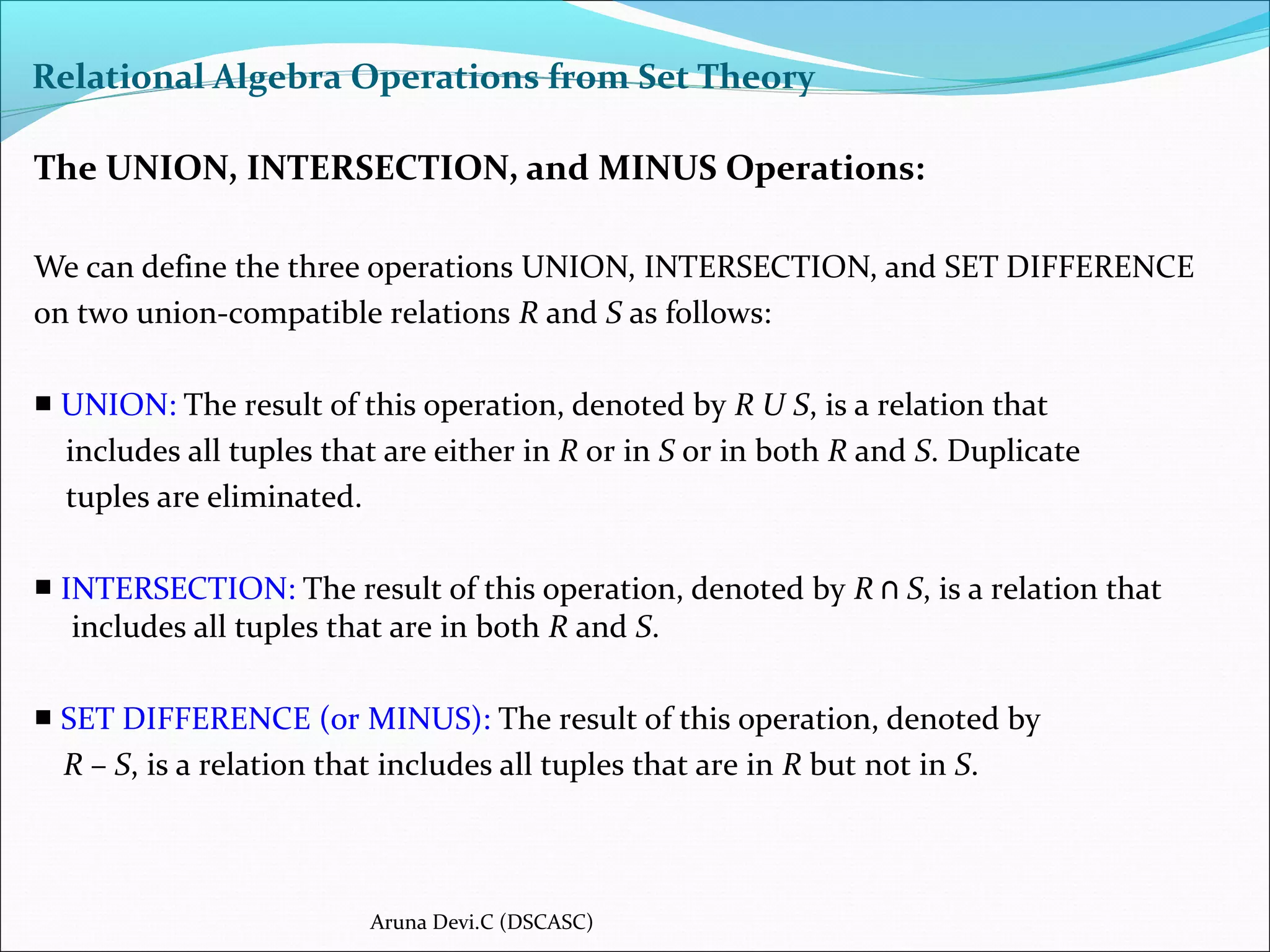
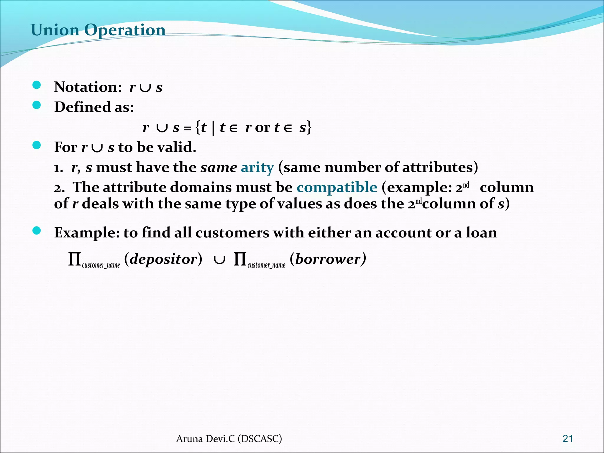
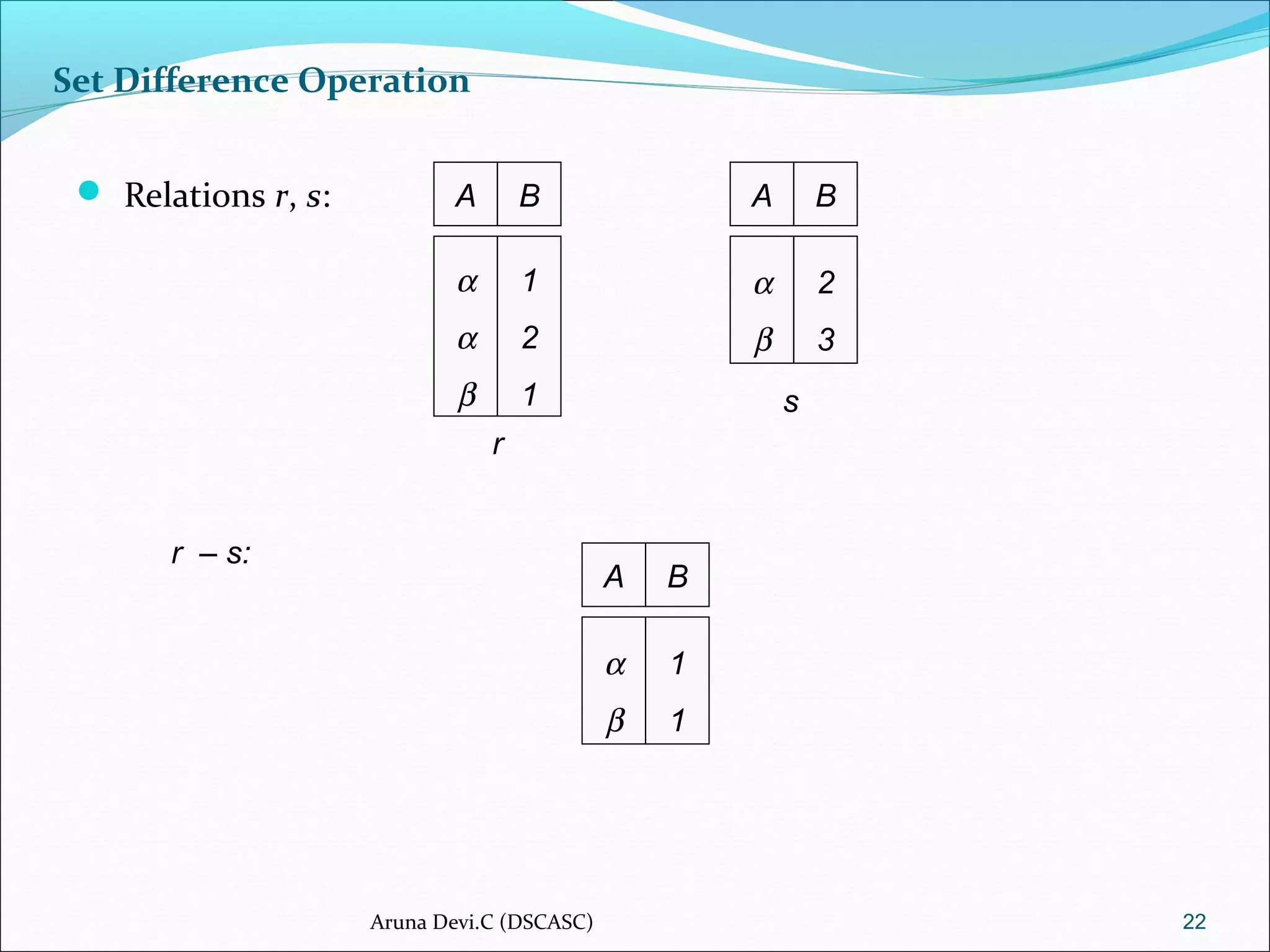
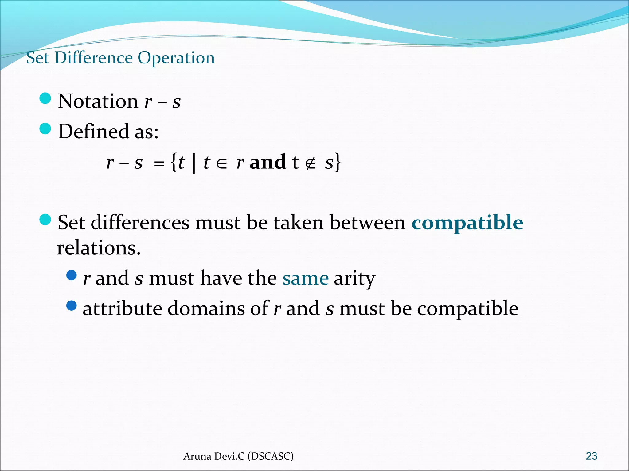
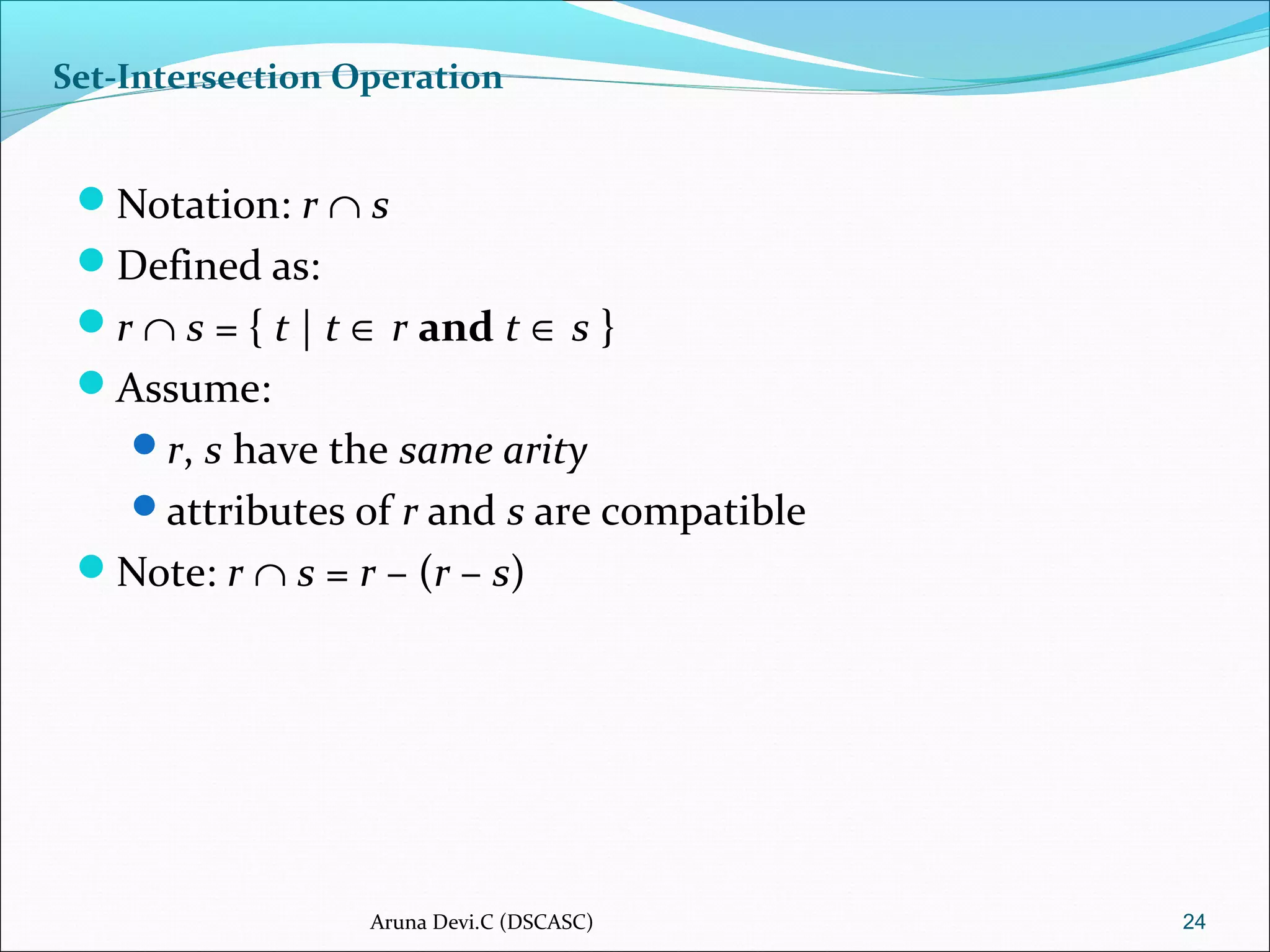
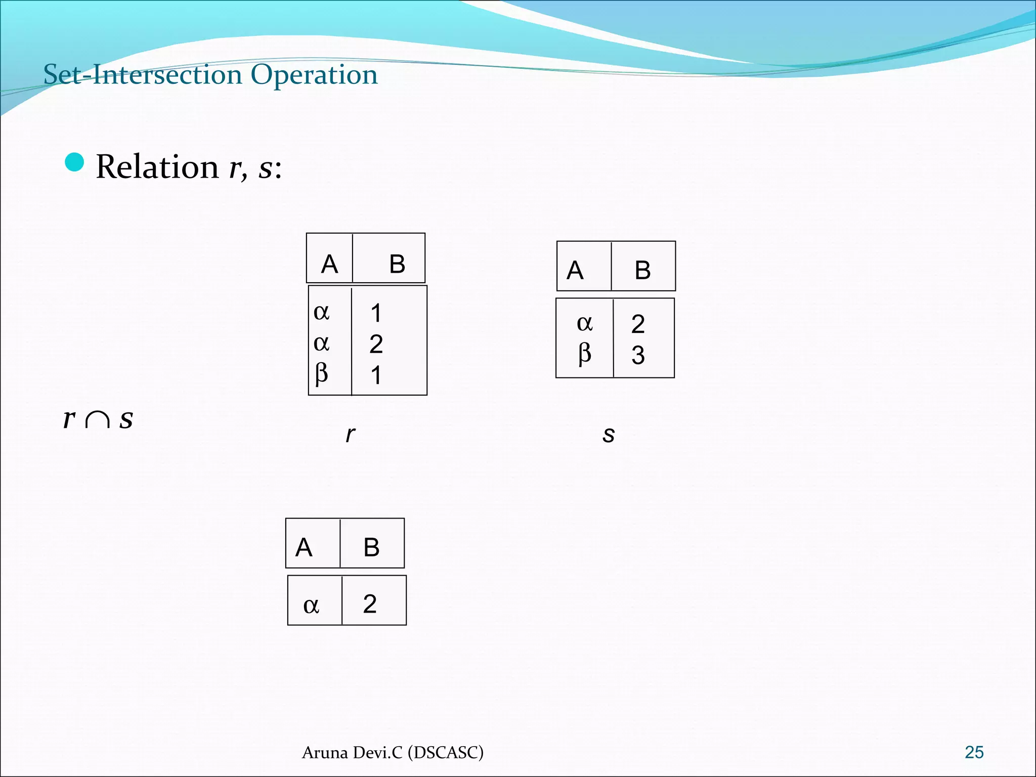
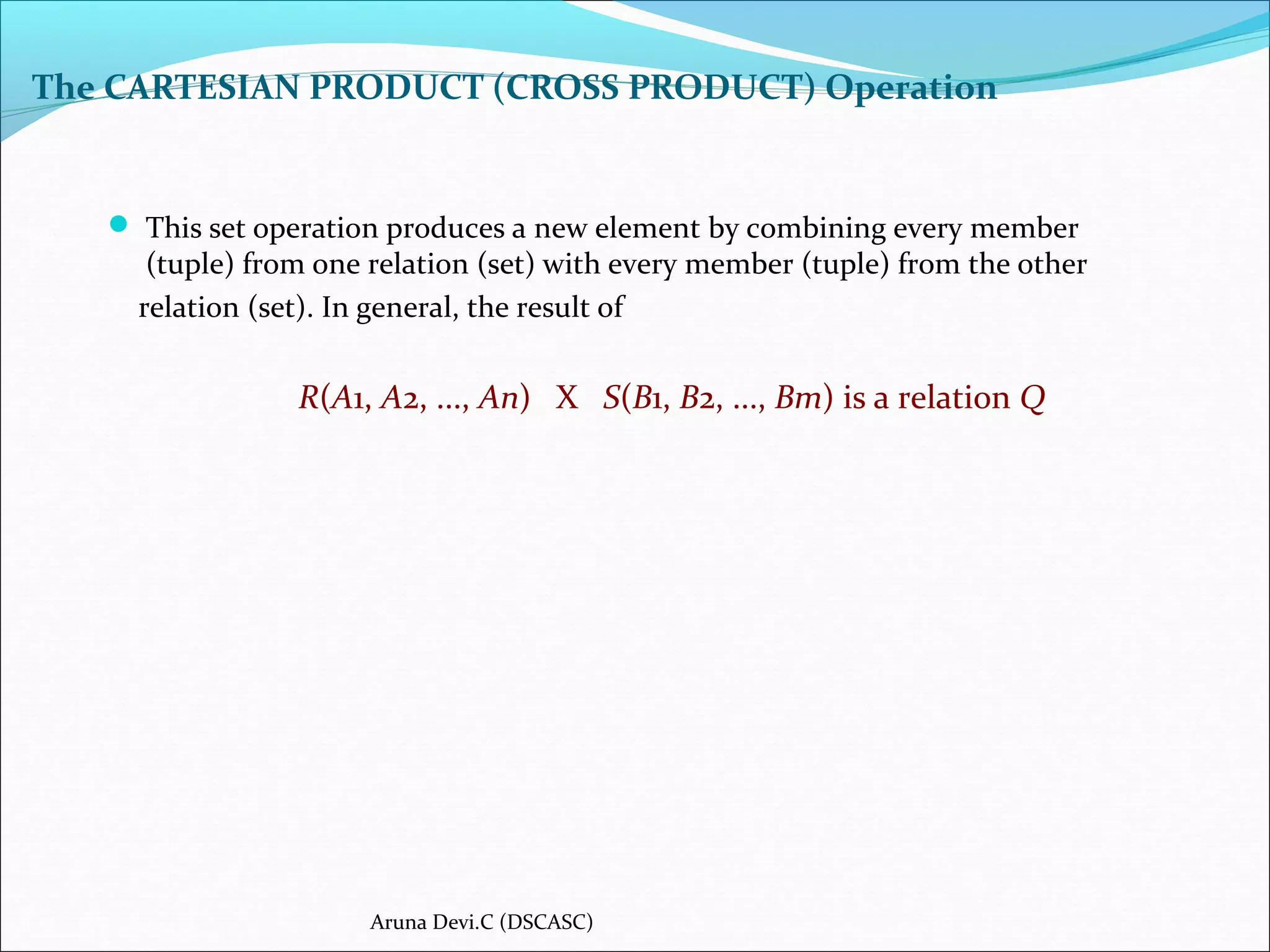
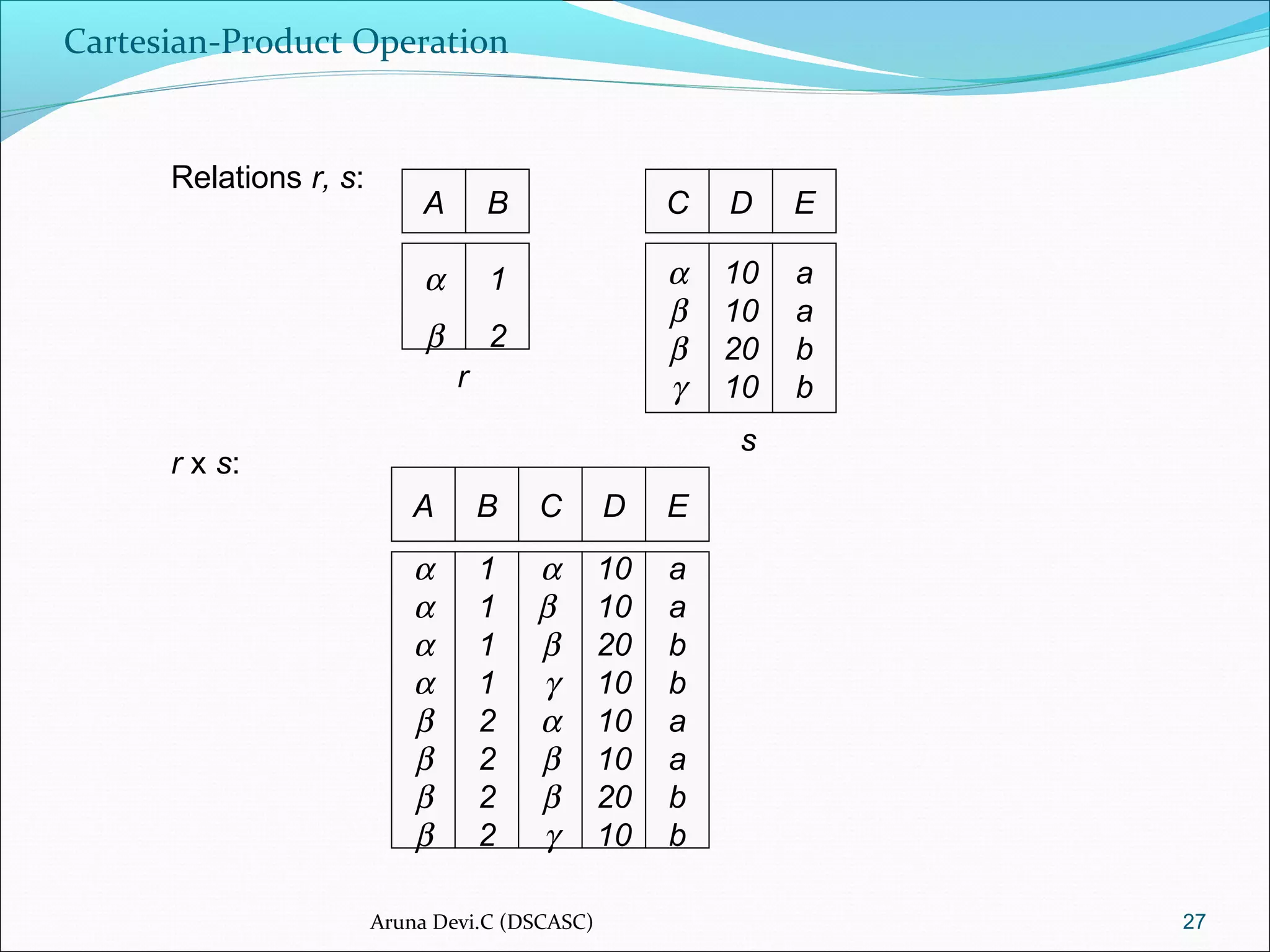
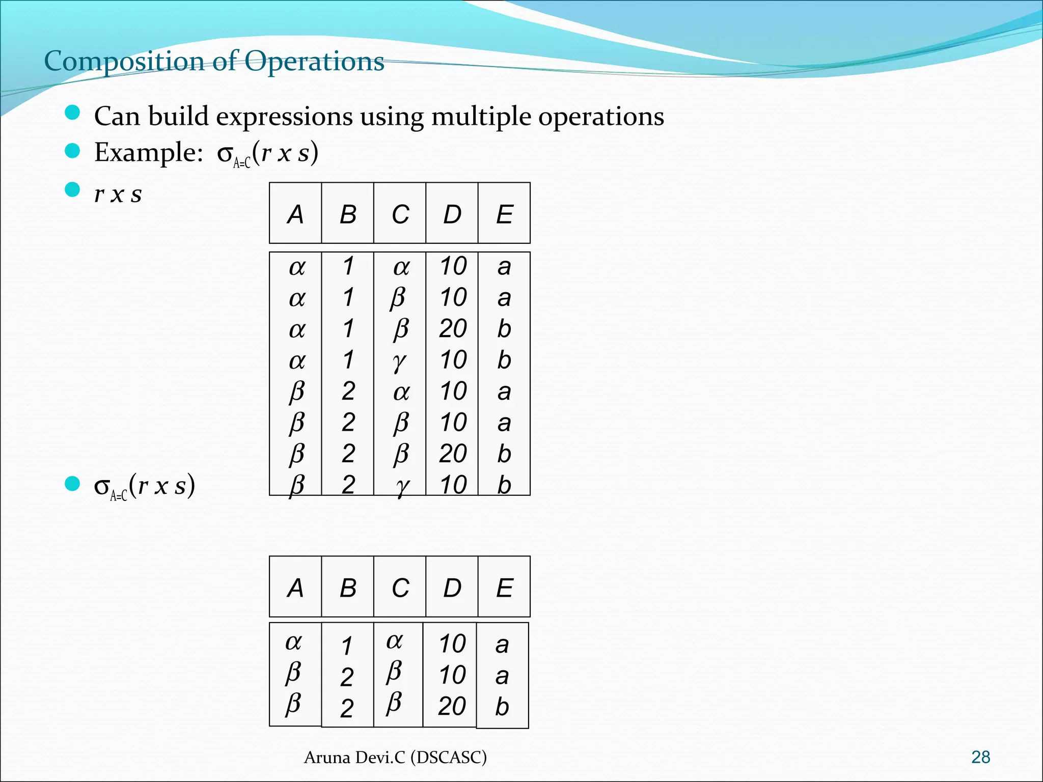
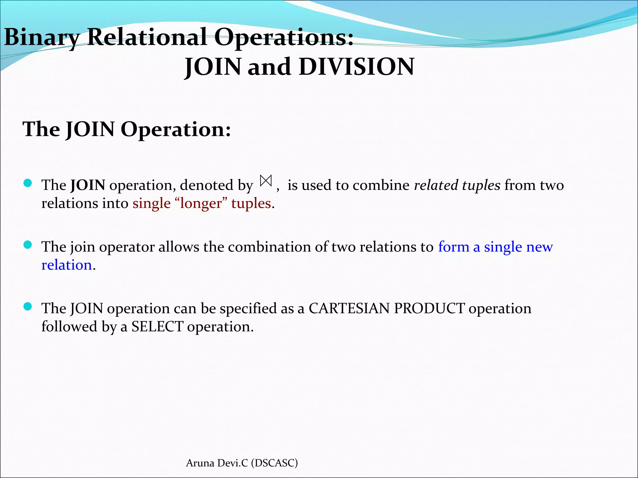
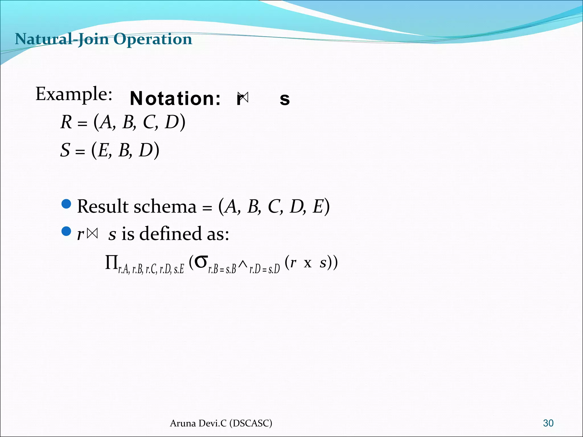
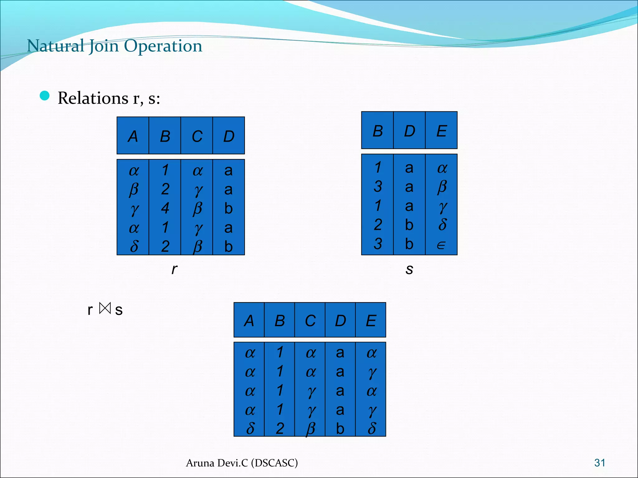
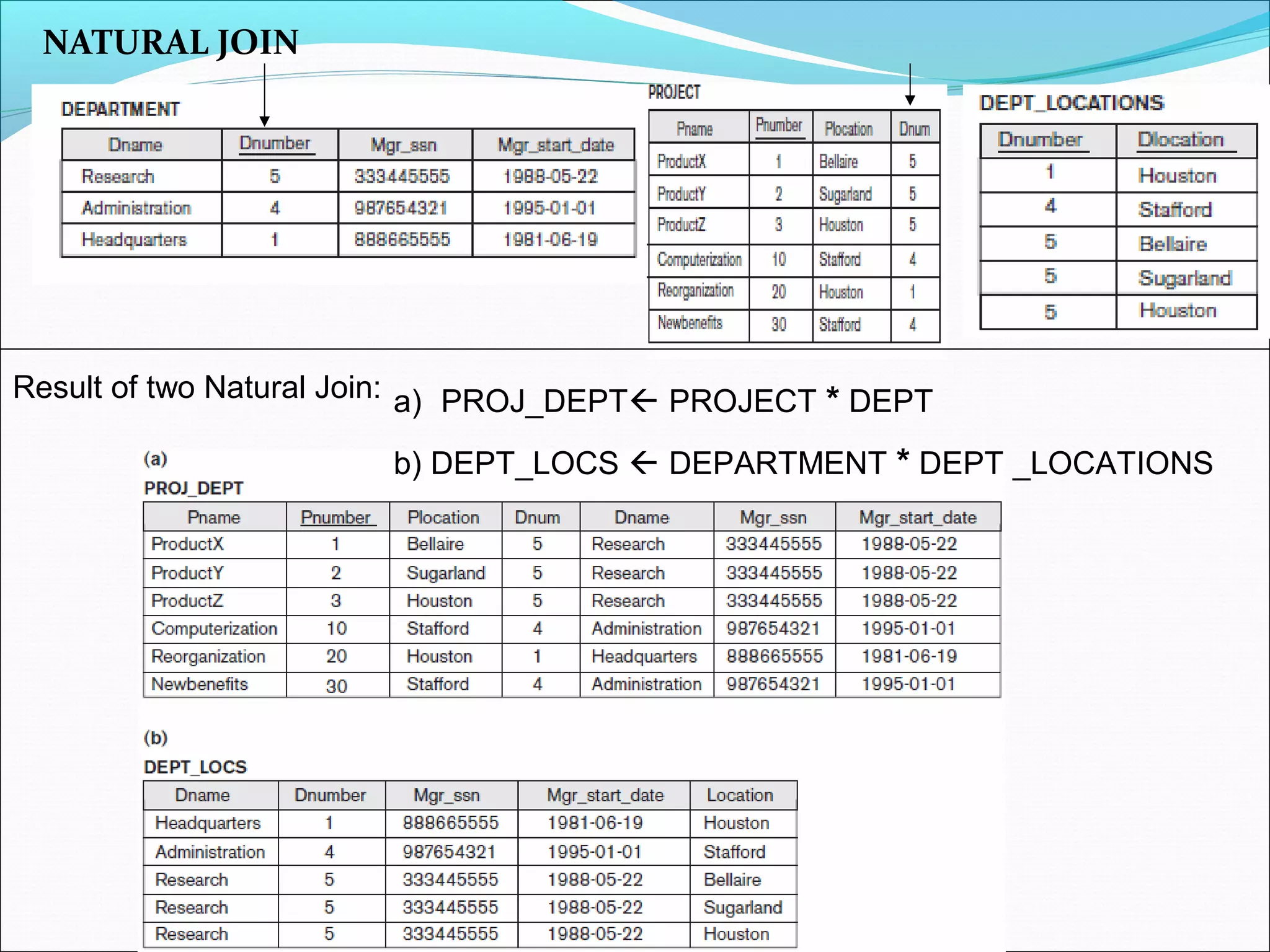
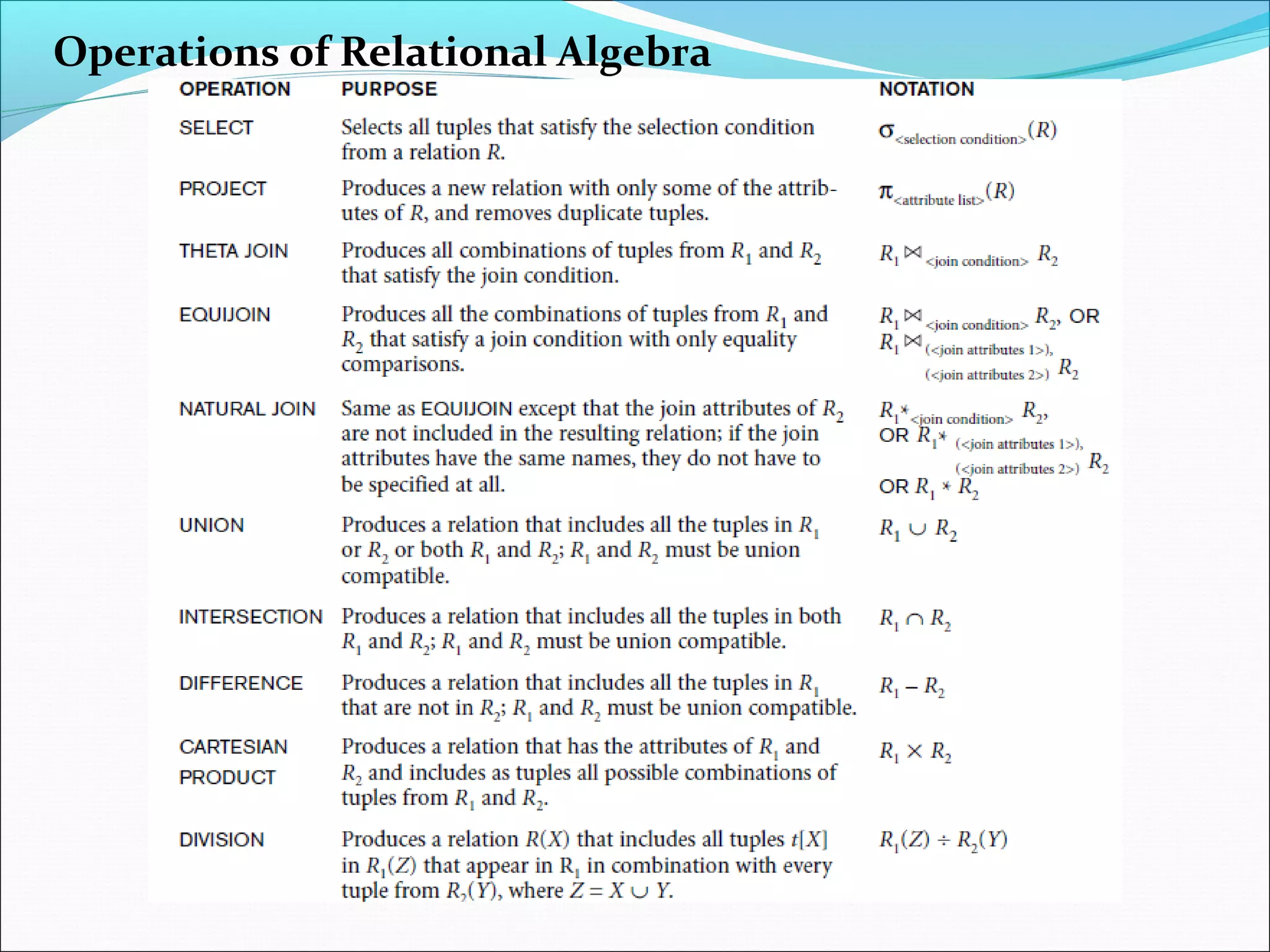
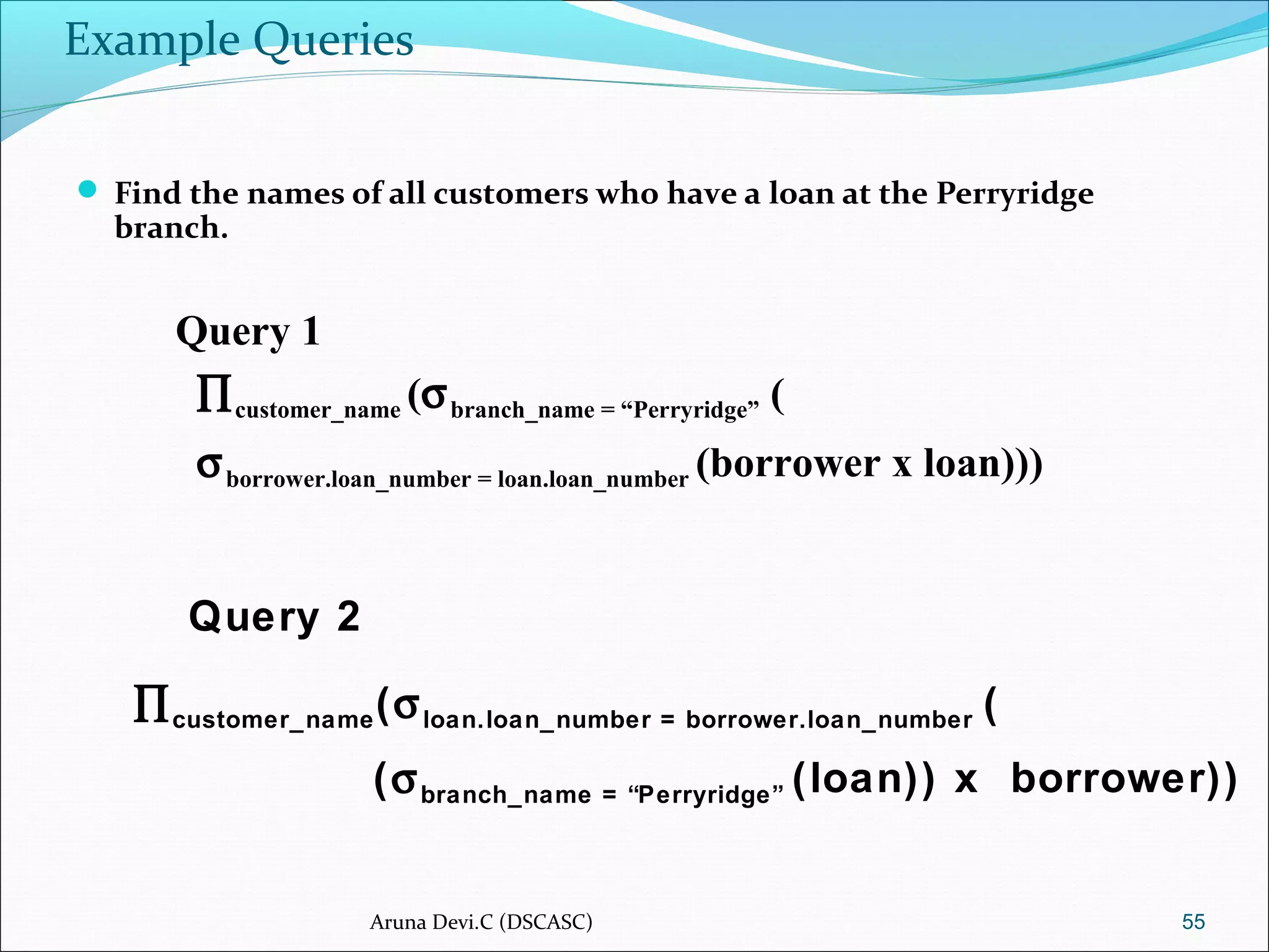
SlideShare a Scribd company logo
Aruna Devi.C (DSCASC) 1
Data Base Management System
[DBMS]
Chapter 5
Unit III
Relational Algebra
Relational Algebra
 Historically, the relational algebra and calculus were developed before the SQL
language.
 In fact, in some ways, SQL is based on concepts from both the algebra and the
calculus.
 The algebra defines a set of operations for the relational model.
 A relational calculus expression creates a new relation.
Aruna Devi.C (DSCASC)
 The relational algebra is often considered to be an integral part of the relational
data model.
Its operations can be divided into two groups:
 First group - set operations from mathematical set theory; these are applicable
because each relation is defined to be a set of tuples in the formal relational
model.
 Set operations include UNION, INTERSECTION, SET DIFFERENCE, and
CARTESIAN PRODUCT (also known as CROSS PRODUCT).
 Second group - consists of operations developed specifically for relational
databases—these include SELECT, PROJECT, and JOIN, among others.
Relational Algebra (cont.,)
Aruna Devi.C (DSCASC)
Relational Algebra
Six basic operators:
Select: σ - Selects tuples that satisfy a given predicate
Project: ∏ - Projects specified fields.
Union: ∪
Intersection: ∩
Set difference: –
Cartesian product: x
Rename: ρ
Division: ÷
Joints
The operators take one or two relations as inputs and produce a
new relation as a result.
4Aruna Devi.C (DSCASC)
Unary Relational Operations
SELECT and PROJECT
The SELECT Operation:
 The SELECT operation is used to choose a subset of the tuples from a relation that
satisfies a selection condition.
 The SELECT operation is denoted by
σ <selection condition> (R)
where the symbol σ (sigma) is used to denote the SELECT operator.
 The selection condition is a Boolean expression (condition) specified on the
attributes of relation R.
 σ Dno=4(EMPLOYEE)
 σ Salary>30000(EMPLOYEE)
Where Dno is Department
No.
 <comparison op> is normally one of the operators {=, <, ≤, >, ≥, ≠}.
 Clauses can be connected by the standard Boolean operators and, or, and not to
form a general selection condition.
Select Operation
 Notation: σ p(r)
 p is called the selection predicate
 Defined as:
σP(r) = {t | t ∈ r and p(t)}
Where p is a formula connected by : ∧ (and), ∨ (or), ¬ (not)
Example of selection:
σ branch_name=“Perryridge”(account)
6Aruna Devi.C (DSCASC)
Select Operation – Example
7
Relation r
A B C D
α
α
β
β
α
β
β
β
1
5
12
23
7
7
3
10
σA=B ^ D > 5 (r)
A B C D
α
β
α
β
1
23
7
10
Aruna Devi.C (DSCASC)
The PROJECT Operation:
 The PROJECT operation, selects certain columns from the table and discards the
other columns.
 The SELECT operation chooses some of the rows from the table while discarding
other rows.
 The general form of the PROJECT operation is
π <attribute list> (R)
where π (pi) is the symbol used to represent the PROJECT operation, and <attribute
list> is the desired sublist of attributes from the attributes of relation R.
For example, to list each employee’s first and last name and salary, we can use the
PROJECT operation as follows:
π Lname, Fname, Salary(EMPLOYEE)
Unary Relational Operations
SELECT and PROJECT
Project Operation
 Notation:
where A1, A2 are attribute names and r is a relation name.
 The result is defined as the relation of k columns obtained by erasing the
columns that are not listed.
 Duplicate rows removed from result, since relations are sets
Eg: To eliminate the branch_name attribute of account
∏account_number,balance (account)
9
)(,,, 21
rkAAA 
∏
Aruna Devi.C (DSCASC)
Project Operation – Example
Relation r:
10
A B C
α
α
β
β
10
20
30
40
1
1
1
2
A C
α
α
β
β
1
1
1
2
=
A C
α
β
β
1
1
2
∏A,C (r)
Aruna Devi.C (DSCASC)
SELECT and PROJECT
Aruna Devi.C (DSCASC)
Company Database
SELECT and PROJECT
 In SQL, the SELECT condition is typically specified in the WHERE clause of a
query.
 For example, the following operation:
σDno=4 AND Salary>25000 (EMPLOYEE)
would correspond to the following SQL query:
SELECT * FROM EMPLOYEE WHERE Dno=4 AND Salary>25000;
Aruna Devi.C (DSCASC)
Company Database
Sequences of Operations
 To retrieve the first name, last name, and salary of all employees who work in
department number 5, we must apply a SELECT and a PROJECT operation.
 We can write a single relational algebra expression, also known as an in-line
expression, as follows:
π Fname, Lname, Salary(σDno=5(EMPLOYEE))
Next page shows the result of this in-line relational algebra expression.
Aruna Devi.C (DSCASC)
Sequences of Operations
π Fname, Lname, Salary(σDno=5(EMPLOYEE))
Aruna Devi.C (DSCASC)
Company Database
Sequences of Operations
 To rename the attributes in a relation, we simply list the new attribute names in
parentheses, as in the following example:
TEMP σDno=5(EMPLOYEE)←
R(First_name, Last_name, Salary) πFname, Lname, Salary(TEMP)←
 If no renaming is applied, the names of the attributes in the resulting relation of a
SELECT operation are the same as those in the original relation and in the same
order.
 For a PROJECT operation with no renaming, the resulting relation has the same
attribute names as those in the projection list and in the same order in which they
appear in the list.
Aruna Devi.C (DSCASC)
Sequences of Operations
TEMP ← σDno=5(EMPLOYEE)
R(First_name, Last_name, Salary) ← πFname, Lname, Salary(TEMP)
Aruna Devi.C (DSCASC)
Company Database
Rename Operation
 Allows us to name, and therefore to refer to, the results of relational-algebra
expressions.
 Allows us to refer to a relation by more than one name.
Example:
ρ x (E)
returns the expression E under the name X
 If a relational-algebra expression E has arity n, then returns the result of
expression E under the name X, and with the attributes renamed to A1, A2, ….,
An.
17
)(),...,,( 21
EnAAAx
ρ
Aruna Devi.C (DSCASC)
Rename Operation
 In SQL, a single query typically represents a complex relational algebra
expression.
 Renaming in SQL is accomplished by aliasing using AS, as in the following
example:
 SELECT E.Fname AS First_name, E.Lname AS Last_name, E.Salary AS Salary
FROM EMPLOYEE AS E
WHERE E.Dno=5,
Aruna Devi.C (DSCASC)
Company Database
Union Operation – Example
 Relations r, s:
19
r ∪ s:
A B
α
α
β
1
2
1
A B
α
β
2
3
r
s
A B
α
α
β
β
1
2
1
3
Aruna Devi.C (DSCASC)
Relational Algebra Operations from Set Theory
The UNION, INTERSECTION, and MINUS Operations:
We can define the three operations UNION, INTERSECTION, and SET DIFFERENCE
on two union-compatible relations R and S as follows:
■ UNION: The result of this operation, denoted by R U S, is a relation that
includes all tuples that are either in R or in S or in both R and S. Duplicate
tuples are eliminated.
■ INTERSECTION: The result of this operation, denoted by R ∩ S, is a relation that
includes all tuples that are in both R and S.
■ SET DIFFERENCE (or MINUS): The result of this operation, denoted by
R – S, is a relation that includes all tuples that are in R but not in S.
Aruna Devi.C (DSCASC)
Union Operation
 Notation: r ∪ s
 Defined as:
r ∪ s = {t | t ∈ r or t ∈ s}
 For r ∪ s to be valid.
1. r, s must have the same arity (same number of attributes)
2. The attribute domains must be compatible (example: 2nd
column
of r deals with the same type of values as does the 2nd
column of s)
 Example: to find all customers with either an account or a loan
∏customer_name (depositor) ∪ ∏customer_name (borrower)
21Aruna Devi.C (DSCASC)
Set Difference Operation
 Relations r, s:
22
r – s:
A B
α
α
β
1
2
1
A B
α
β
2
3
r
s
A B
α
β
1
1
Aruna Devi.C (DSCASC)
Set Difference Operation
Notation r – s
Defined as:
r – s = {t | t ∈ r and t ∉ s}
Set differences must be taken between compatible
relations.
r and s must have the same arity
attribute domains of r and s must be compatible
23Aruna Devi.C (DSCASC)
Set-Intersection Operation
Notation: r ∩ s
Defined as:
r ∩ s = { t | t ∈ r and t ∈ s }
Assume:
r, s have the same arity
attributes of r and s are compatible
Note: r ∩ s = r – (r – s)
24Aruna Devi.C (DSCASC)
Set-Intersection Operation
Relation r, s:
r ∩ s
25
A B
α
α
β
1
2
1
A B
α
β
2
3
r s
A B
α 2
Aruna Devi.C (DSCASC)
The CARTESIAN PRODUCT (CROSS PRODUCT) Operation
 This set operation produces a new element by combining every member
(tuple) from one relation (set) with every member (tuple) from the other
relation (set). In general, the result of
R(A1, A2, ..., An) X S(B1, B2, ..., Bm) is a relation Q
Aruna Devi.C (DSCASC)
Cartesian-Product Operation
27
Relations r, s:
r x s:
A B
α
β
1
2
A B
α
α
α
α
β
β
β
β
1
1
1
1
2
2
2
2
C D
α
β
β
γ
α
β
β
γ
10
10
20
10
10
10
20
10
E
a
a
b
b
a
a
b
b
C D
α
β
β
γ
10
10
20
10
E
a
a
b
br
s
Aruna Devi.C (DSCASC)
Composition of Operations
 Can build expressions using multiple operations
 Example: σA=C(r x s)
 r x s
 σA=C(r x s)
28
A B
α
α
α
α
β
β
β
β
1
1
1
1
2
2
2
2
C D
α
β
β
γ
α
β
β
γ
10
10
20
10
10
10
20
10
E
a
a
b
b
a
a
b
b
A B C D E
α
β
β
1
2
2
α
β
β
10
10
20
a
a
b
Aruna Devi.C (DSCASC)
Binary Relational Operations:
JOIN and DIVISION
The JOIN Operation:
 The JOIN operation, denoted by , is used to combine related tuples from two
relations into single “longer” tuples.
 The join operator allows the combination of two relations to form a single new
relation.
 The JOIN operation can be specified as a CARTESIAN PRODUCT operation
followed by a SELECT operation.
Aruna Devi.C (DSCASC)
Natural-Join Operation
Example:
R = (A, B, C, D)
S = (E, B, D)
Result schema = (A, B, C, D, E)
r s is defined as:
∏r.A,r.B,r.C,r.D,s.E (σr.B=s.B∧r.D=s.D (r x s))
30
Notation: r s
Aruna Devi.C (DSCASC)
Natural Join Operation
Relations r, s:
31
A B
α
β
γ
α
δ
1
2
4
1
2
C D
α
γ
β
γ
β
a
a
b
a
b
B
1
3
1
2
3
D
a
a
a
b
b
E
α
β
γ
δ
∈
r
A B
α
α
α
α
δ
1
1
1
1
2
C D
α
α
γ
γ
β
a
a
a
a
b
E
α
γ
α
γ
δ
s
r s
Aruna Devi.C (DSCASC)
Variations of JOIN: The EQUIJOIN and NATURAL JOIN
 The only comparison operator used is =, is called an EQUIJOIN.
 NATURAL JOIN requires that the two join attributes (or each pair of join attributes)
have the same name in both relations.
 The equality join condition specified on these two attributes requires the values to be
identical in every tuple in the result.
 NATURAL JOIN — denoted by *— was created to get rid of the second (superfluous)
attribute in an EQUIJOIN condition.
Aruna Devi.C (DSCASC)
COMPANY Relational database schema
Join Operation
Result of Join Operation:
DEPT_MGR  DEPARTMENT Mgr_ssn= ssn EMPLOYEE
NATURAL JOIN
Result of two Natural Join: a) PROJ_DEPT PROJECT * DEPT
b) DEPT_LOCS  DEPARTMENT * DEPT _LOCATIONS
A Complete Set of Relational Algebra Operations
Relational algebra operations {σ, π, U, ρ, –, x} is a complete set.
 For example, the INTERSECTION operation can be expressed by using UNION
and MINUS.
 A JOIN operation can be specified as a CARTESIAN PRODUCT followed by a
SELECT operation.
 A NATURAL JOIN can be specified as a CARTESIAN PRODUCT preceded by
RENAME and followed by SELECT and PROJECT operations.
Aruna Devi.C (DSCASC)
A Complete Set of Relational Algebra Operations (Cont.,)
 An example is Retrieve the names of employees who work on all the projects
that ‘John Smith’ works on.
 First, retrieve the list of project numbers that ‘John Smith’ works on in the
intermediate relation SMITH_PNOS:
Aruna Devi.C (DSCASC)
Division Operation
 The DIVISION operation, denoted by ÷, is useful for a special kind of query that
sometimes occurs in database applications.
 An example is Retrieve the names of employees who work on all the projects that
‘John Smith’ works on.
1) First, retrieve the list of project numbers that ‘John Smith’ works on in the
intermediate relation SMITH_PNOS:
SMITH ← σFname=‘John’ AND Lname=‘Smith’ (EMPLOYEE)
SMITH_PNOS ← πPno (WORKS_ON Essn=Ssn SMITH)
2) Next, create a relation that includes a tuple <Pno, Essn> whenever the employee
whose Ssn is Essn works on the project whose number is Pno in the intermediate
relation SSN_PNOS:
SSN_PNOS ← πEssn, Pno (WORKS_ON)
38Aruna Devi.C (DSCASC)
Company Database
Division Operation
3) Finally, apply the DIVISION operation to the two relations, which gives the desired
employees’ Social Security numbers:
SSNS(Ssn) SSN_PNOS← ÷ SMITH_PNOS
RESULT πFname, Lname (SSNS← * EMPLOYEE)
Company Database
Division Operation
In general, the DIVISION operation is applied to two
relations R(Z) ÷ S(X), where the attributes of R are a subset of
the attributes of S.
Example:
1) The table SSN_PNOS is from works on table.
2)The table Smith-Pnos is from which project smith work-on, that is from employee table and
works-on table.
3) SSNS is the final table where check which all projects smith the same projects all the other
employees should work on so only two employees work for both the projects.
Aruna Devi.C (DSCASC)
Operations of Relational Algebra
Additional Relational Operations
1. Generalized Projection:
 The generalized projection operation extends the projection operation by allowing
functions of attributes to be included in the projection list.
 The generalized form can be expressed as:
πF1, F2, ..., Fn (R)
where F1, F2, ..., Fn are functions over the attributes in relation R and may involve
arithmetic operations and constant values.
 This operation is helpful when developing reports where computed values have to be
produced in the columns of a query result.
Aruna Devi.C (DSCASC)
Additional Relational Operations (Cont.,)
 As an example, consider the relation
EMPLOYEE (Ssn, Salary, Deduction, Years_service)
 A report may be required to show
Net Salary = Salary – Deduction,
Bonus = 2000 * Years_service, and
Tax = 0.25 * Salary.
 Then a generalized projection combined with renaming may be used as follows:
REPORT ρ(Ssn, Net_salary, Bonus, Tax)(πSsn, Salary – Deduction, 2000 * Years_service, 0.25 * Salary(EMPLOYEE))←
Aruna Devi.C (DSCASC)
2. Aggregate Functions and Grouping:
 Another type of request that cannot be expressed in the basic relational algebra is to
specify mathematical aggregate functions on collections of values from the database.
 Examples: Retrieving the average or total salary of all employees or the total number of
employee tuples.
 Common functions applied to collections of numeric values include SUM, AVERAGE,
MAXIMUM, MINIMUM and COUNT.
 Another common type of request involves grouping the tuples in a relation.
 Example: Group EMPLOYEE tuples by Dno.
Additional Relational Operations (Cont.,)
Aruna Devi.C (DSCASC)
Additional Relational Operations (Cont.,)
 We can define an AGGREGATE FUNCTION operation, using the symbol .ℑ
<grouping attributes> <function list> (ℑ R)
Example:
Aruna Devi.C (DSCASC)
Additional Relational Operations (Cont.,)
3. Recursive Closure Operations:
This operation is applied to a recursive relationship
between tuples of the same type, such as the relationship
between an employee and a supervisor.
Aruna Devi.C (DSCASC)
Additional Relational Operations (Cont.,)
4. OUTER JOIN Operations:
 The JOIN operations described earlier match tuples that satisfy the join
condition.
 For example, for a NATURAL JOIN operation R * S, only tuples from R that have
matching tuples in S—and vice versa—appear in the result.
 Hence, tuples without a matching (or related) tuple are eliminated from the
JOIN result.
 Tuples with NULL values in the join attributes are also eliminated.
 This type of join, where tuples with no match are eliminated, is known as an
inner join.
 There is an amount of loss in information.
Aruna Devi.C (DSCASC)
Additional Relational Operations (Cont.,)
Different JOINs:
 Join: Return rows when there is at least one match in both tables.
 Left Outer Join: Return all rows from the first or left table, even if there are no
matches in the right table. R S
 Right Outer Join: Return all rows from the second or right table, even if there
are no matches in the left table. R S
 Full Outer Join: Return rows when there is a match in one of the tables.
R S
Aruna Devi.C (DSCASC)
Examples of Queries in Relational Algebra
Examples of Queries in Relational Algebra (Cont.,)
 Query 1. Retrieve the name and address of all employees who work for the ‘Research’
department.
 Query 2. For every project located in ‘Stafford’, list the project number, the controlling
department number, and the department manager’s last name, address, and birth date.
 we first select the projects located in Stafford, then join them with their controlling departments, and then
join the result with the department managers. Finally, we apply a project operation on the desired
attributes.
 Query 3. Find the names of employees who work on all the projects controlled by
department number 5.
 In this query, we first create a table DEPT5_PROJS that contains the project
numbers of all projects controlled by department 5.
 Then we create a table EMP_PROJ that holds (Ssn, Pno) tuples, and apply the
division operation.
 Notice that we renamed the attributes so that they will be correctly used in the
division operation.
 Finally,we join the result of the division, which holds only Ssn values, with the
EMPLOYEE table to retrieve the desired attributes from EMPLOYEE.
Examples of Queries in Relational Algebra (Cont.,)
Aruna Devi.C (DSCASC)
 Query 4. Make a list of project numbers for projects that involve an employee
whose last name is ‘Smith’, either as a worker or as a manager of the department
that controls the project.
 In this query, we retrieved the project numbers for projects that involve an
employee named Smith as a worker in SMITH_WORKER_PROJS. Then we
retrieved the project numbers for projects that involve an employee named Smith
as manager of the department that controls the project in SMITH_MGR_PROJS.
Finally, we applied the UNION operation on SMITH_WORKER_PROJS and
SMITH_MGR_PROJS.
Examples of Queries in Relational Algebra (Cont.,)
Aruna Devi.C (DSCASC)
Other Example Queries
 Find all loans of over $1200
53
Find the loan number for each loan of an amount greater
than $1200
σamount > 1200 (loan)
∏loan_number (σamount > 1200 (loan))
 Find the names of all customers who have a loan, an
account, or both, from the bank
Find the names of all customers who have a loan
and an account at bank.
∏customer_name (borrower) ∪ ∏customer_name (depositor)
∏customer_name (borrower) ∩ ∏customer_name
(depositor)
Example Queries
1) Find the names of all customers who have a loan at the Perryridge
branch.
54
2) Find the names of all customers who have a loan at the Perryridge
branch but do not have an account at any branch of the bank.
∏customer_name (σbranch_name = “Perryridge”
(σborrower.loan_number = loan.loan_number(borrower x loan))) –
∏customer_name(depositor)
∏customer_name (σbranch_name=“Perryridge”
(σborrower.loan_number = loan.loan_number(borrower x loan)))
Aruna Devi.C (DSCASC)
Example Queries
 Find the names of all customers who have a loan at the Perryridge
branch.
55
Query 2
∏customer_name(σloan.loan_number = borrower.loan_number (
(σbranch_name = “Perryridge” (loan)) x borrower))
Query 1
∏customer_name (σbranch_name = “Perryridge” (
σborrower.loan_number = loan.loan_number (borrower x loan)))
Aruna Devi.C (DSCASC)
Relational Database Design Using
ER-to-Relational Mapping
Chapter 6
Step 1: Mapping of Regular Entity Types.
Step 2: Mapping of Weak Entity Types.
Step 3: Mapping of Binary 1:1 Relationship Types.
Step 4: Mapping of Binary 1:N Relationship Types.
Step 5: Mapping of Binary M:N Relationship Types.
Step 6: Mapping of Multi valued Attributes.
Step 7: Mapping of N-ary Relationship Types.
Relational Database Design Using ER-to-Relational Mapping (Cont.,)
Step 1: Mapping of Regular Entity Types:
 For each regular (strong) entity type E in the ER schema, create a relation R that
includes all the simple attributes of E.
 Include only the simple component attributes of a composite attribute.
 Choose one of the key attributes of E as the primary key for R.
 If the chosen key of E is a composite, then the set of simple attributes that form it
will together form the primary key of R.
 If multiple keys were identified for E during the conceptual design, the information
describing the attributes that form each additional key is kept in order to specify
secondary (unique) keys of relation R.
 We create the relations EMPLOYEE, DEPARTMENT, and PROJECT in Figure 2 to
correspond to the regular entity types EMPLOYEE, DEPARTMENT, and PROJECT in
Figure 1.
Relational Database Design Using ER-to-Relational Mapping (Cont.,)
 The foreign key and relationship attributes, if any, are not included yet; they will
be added during subsequent steps.
 Example, we choose Ssn, Dnumber, and Pnumber as primary keys for the
relations EMPLOYEE, DEPARTMENT, and PROJECT, respectively.
 The relations that are created from the mapping of entity types are sometimes
called entity relations because each tuple represents an entity instance.
Relational Database Design Using ER-to-Relational Mapping
ER-to-Relational Mapping Algorithm:
Relational Database Design Using ER-to-Relational Mapping (Cont.,)
Step 2: Mapping of Weak Entity Types:
 For each weak entity type W in the ER schema with owner entity type E, create a
relation R and include all simple attributes (or simple components of composite
attributes) of W as attributes of R.
 In addition, include as foreign key attributes of R, the primary key attribute(s) of
the relation(s) that correspond to the owner entity type(s); this takes care of
mapping the identifying relationship type of W.
 The primary key of R is the combination of the primary key(s) of the owner(s) and
the partial key of the weak entity type W, if any.
Aruna Devi.C (DSCASC)
Relational Database Design Using ER-to-Relational Mapping (Cont.,)
 We create the relation DEPENDENT in this step to correspond to the weak entity
type DEPENDENT.
 The primary key of the DEPENDENT relation is the combination {Essn,
Dependent_name}, because Dependent_name is the partial key of DEPENDENT.
Aruna Devi.C (DSCASC)
Relational Database Design Using ER-to-Relational Mapping (Cont.,)
Step 3: Mapping of Binary 1:1 Relationship Types:
 For each binary 1:1 relationship type R in the ER schema, identify the relations S
and T that correspond to the entity types participating in R.
 There are three possible approaches:
(a) the foreign key approach,
(b) the merged relationship approach, and
(c) the cross reference or relationship relation approach.
a. Foreign key approach:
 Choose one of the relations—S, say—and include as a foreign key in S
the primary key of T.
 We include the primary key of the EMPLOYEE relation as foreign key
in the DEPARTMENT relation and rename it Mgr_ssn.
Aruna Devi.C (DSCASC)
Relational Database Design Using ER-to-Relational Mapping (Cont.,)
b. Merged relation approach:
 An alternative mapping of a 1:1 relationship type is to merge the two entity types
and the relationship into a single relation.
c. Cross-reference or relationship relation approach:
 The third option is to set up a third relation R for the purpose of cross-
referencing the primary keys of the two relations S and T representing the entity
types.
Aruna Devi.C (DSCASC)
Relational Database Design Using ER-to-Relational Mapping (Cont.,)
Step 4: Mapping of Binary 1:N Relationship Types:
 For each regular binary 1:N relationship type R, identify the relation S that
represents the participating entity type at the N-side of the relationship type.
 Include any simple attributes (or simple components of composite attributes) of
the 1:N relationship type as attributes of S.
 Example, we now map the 1:N relationship types WORKS_FOR, CONTROLS, and
SUPERVISION from Figure 1.
 For WORKS_FOR we include the primary key Dnumber of the DEPARTMENT
relation as foreign key in the EMPLOYEE relation and call it Dno.
 For SUPERVISION we include the primary key of the EMPLOYEE relation as
foreign key in the EMPLOYEE relation itself—because the relationship is
recursive— and call it Super_ssn.
Relational Database Design Using ER-to-Relational Mapping (Cont.,)
Step 5: Mapping of Binary M:N Relationship Types:
 For each binary M:N relationship type R, create a new relation S to represent R.
 Include as foreign key attributes in S the primary keys of the relations that
represent the participating entity types; their combination will form the primary
key of S.
 Example, we map the M:N relationship type WORKS_ON from Figure 1 by
creating the relation WORKS_ON in Figure 2.
 We include the primary keys of the PROJECT and EMPLOYEE relations as foreign
keys in WORKS_ON and rename them Pno and Essn, respectively.
Relational Database Design Using ER-to-Relational Mapping (Cont.,)
Step 6: Mapping of Multi valued Attributes:
 For each multi valued attribute A, create a new relation R.
 This relation R will include an attribute corresponding to A, plus the primary key
attribute K—as a foreign key in R—of the relation that represents the entity type
or relationship type that has A as a multi valued attribute.
 The primary key of R is the combination of A and K.
 Example, we create a relation DEPT_LOCATIONS.
Aruna Devi.C (DSCASC)
Relational Database Design Using ER-to-Relational Mapping (Cont.,)
 The attribute Dlocation represents the multivalued attribute LOCATIONS of
DEPARTMENT, while Dnumber—as foreign key—represents the primary key
of the DEPARTMENT relation.
 The primary key of DEPT_LOCATIONS is the combination of {Dnumber,
Dlocation}.
Aruna Devi.C (DSCASC)
Relational Database Design Using ER-to-Relational Mapping (Cont.,)
Step 7: Mapping of N-ary Relationship Types:
 For each n-ary relationship type R, where n > 2, create a new relation S to
represent R.
 Include as foreign key attributes in S the primary keys of the relations that
represent the participating entity types.
 The primary key of S is usually a combination of all the foreign keys that
reference the relations representing the participating entity types.
Aruna Devi.C (DSCASC)
Summary of Mapping constructs and constraints
Table : Correspondence between ER and Relational Models
ER Model Relational Model
Entity type “Entity” relation
1:1 or 1:N relationship type Foreign key (or “relationship” relation)
M:N relationship type “Relationship” relation and two foreign keys
n-ary relationship type “Relationship” relation and n foreign keys
Simple attribute Attribute
Composite attribute Set of simple component attributes
Multivalued attribute Relation and foreign key
Value set Domain
Key attribute Primary (or secondary) key
Aruna Devi.C (DSCASC)

More Related Content

What's hot

joins in database
 joins in database joins in database
joins in database
Sultan Arshad
 
14. Query Optimization in DBMS
14. Query Optimization in DBMS14. Query Optimization in DBMS
14. Query Optimization in DBMSkoolkampus
 
Unit iv(simple code generator)
Unit iv(simple code generator)Unit iv(simple code generator)
Unit iv(simple code generator)
Kalaimathi Vijayakumar
 
DBMS: Types of keys
DBMS:  Types of keysDBMS:  Types of keys
DBMS: Types of keys
Bharati Ugale
 
Normalization in DBMS
Normalization in DBMSNormalization in DBMS
Normalization in DBMS
Prateek Parimal
 
Kleene's theorem
Kleene's theoremKleene's theorem
Kleene's theorem
Mobeen Mustafa
 
Greedy Algorithm
Greedy AlgorithmGreedy Algorithm
Greedy Algorithm
Waqar Akram
 
Entity Relationship Diagram
Entity Relationship DiagramEntity Relationship Diagram
Entity Relationship Diagram
Shakila Mahjabin
 
Query Decomposition and data localization
Query Decomposition and data localization Query Decomposition and data localization
Query Decomposition and data localization
Hafiz faiz
 
Compiler Design LR parsing SLR ,LALR CLR
Compiler Design LR parsing SLR ,LALR CLRCompiler Design LR parsing SLR ,LALR CLR
Compiler Design LR parsing SLR ,LALR CLR
Riazul Islam
 
Concurrency control
Concurrency controlConcurrency control
Concurrency control
Soumyajit Dutta
 
Relational algebra in dbms
Relational algebra in dbmsRelational algebra in dbms
Relational algebra in dbmsshekhar1991
 
2.8 normal forms gnf &amp; problems
2.8 normal forms   gnf &amp; problems2.8 normal forms   gnf &amp; problems
2.8 normal forms gnf &amp; problems
Sampath Kumar S
 
Applications of stack
Applications of stackApplications of stack
Applications of stack
eShikshak
 
Dbms Notes Lecture 9 : Specialization, Generalization and Aggregation
Dbms Notes Lecture 9 : Specialization, Generalization and AggregationDbms Notes Lecture 9 : Specialization, Generalization and Aggregation
Dbms Notes Lecture 9 : Specialization, Generalization and Aggregation
BIT Durg
 
FUNCTION DEPENDENCY AND TYPES & EXAMPLE
FUNCTION DEPENDENCY  AND TYPES & EXAMPLEFUNCTION DEPENDENCY  AND TYPES & EXAMPLE
FUNCTION DEPENDENCY AND TYPES & EXAMPLE
Vraj Patel
 
15. Transactions in DBMS
15. Transactions in DBMS15. Transactions in DBMS
15. Transactions in DBMSkoolkampus
 
Dijkstra's algorithm presentation
Dijkstra's algorithm presentationDijkstra's algorithm presentation
Dijkstra's algorithm presentation
Subid Biswas
 
Queue ppt
Queue pptQueue ppt
Queue ppt
SouravKumar328
 

What's hot (20)

joins in database
 joins in database joins in database
joins in database
 
14. Query Optimization in DBMS
14. Query Optimization in DBMS14. Query Optimization in DBMS
14. Query Optimization in DBMS
 
Unit iv(simple code generator)
Unit iv(simple code generator)Unit iv(simple code generator)
Unit iv(simple code generator)
 
DBMS: Types of keys
DBMS:  Types of keysDBMS:  Types of keys
DBMS: Types of keys
 
Normalization in DBMS
Normalization in DBMSNormalization in DBMS
Normalization in DBMS
 
Kleene's theorem
Kleene's theoremKleene's theorem
Kleene's theorem
 
Greedy Algorithm
Greedy AlgorithmGreedy Algorithm
Greedy Algorithm
 
Entity Relationship Diagram
Entity Relationship DiagramEntity Relationship Diagram
Entity Relationship Diagram
 
Np cooks theorem
Np cooks theoremNp cooks theorem
Np cooks theorem
 
Query Decomposition and data localization
Query Decomposition and data localization Query Decomposition and data localization
Query Decomposition and data localization
 
Compiler Design LR parsing SLR ,LALR CLR
Compiler Design LR parsing SLR ,LALR CLRCompiler Design LR parsing SLR ,LALR CLR
Compiler Design LR parsing SLR ,LALR CLR
 
Concurrency control
Concurrency controlConcurrency control
Concurrency control
 
Relational algebra in dbms
Relational algebra in dbmsRelational algebra in dbms
Relational algebra in dbms
 
2.8 normal forms gnf &amp; problems
2.8 normal forms   gnf &amp; problems2.8 normal forms   gnf &amp; problems
2.8 normal forms gnf &amp; problems
 
Applications of stack
Applications of stackApplications of stack
Applications of stack
 
Dbms Notes Lecture 9 : Specialization, Generalization and Aggregation
Dbms Notes Lecture 9 : Specialization, Generalization and AggregationDbms Notes Lecture 9 : Specialization, Generalization and Aggregation
Dbms Notes Lecture 9 : Specialization, Generalization and Aggregation
 
FUNCTION DEPENDENCY AND TYPES & EXAMPLE
FUNCTION DEPENDENCY  AND TYPES & EXAMPLEFUNCTION DEPENDENCY  AND TYPES & EXAMPLE
FUNCTION DEPENDENCY AND TYPES & EXAMPLE
 
15. Transactions in DBMS
15. Transactions in DBMS15. Transactions in DBMS
15. Transactions in DBMS
 
Dijkstra's algorithm presentation
Dijkstra's algorithm presentationDijkstra's algorithm presentation
Dijkstra's algorithm presentation
 
Queue ppt
Queue pptQueue ppt
Queue ppt
 

Viewers also liked

DBMS : Relational Algebra
DBMS : Relational Algebra DBMS : Relational Algebra
DBMS : Relational Algebra
Sridhar Baithi
 
Data integrity Dbms presentation 12 cs 18
Data integrity Dbms presentation 12 cs 18Data integrity Dbms presentation 12 cs 18
Data integrity Dbms presentation 12 cs 18
Engr Imran Ashraf
 
Nested Queries Lecture
Nested Queries LectureNested Queries Lecture
Nested Queries Lecture
Felipe Costa
 
SQL Data Manipulation
SQL Data ManipulationSQL Data Manipulation
SQL Data Manipulation
khalid alkhafagi
 
Normalization case
Normalization caseNormalization case
Normalization case
Prosanta Ghosh
 
Er & eer to relational mapping
Er & eer to relational mappingEr & eer to relational mapping
Er & eer to relational mappingsaurabhshertukde
 
Advanced DBMS presentation
Advanced DBMS presentationAdvanced DBMS presentation
Advanced DBMS presentation
Hindustan Petroleum
 
Acid properties
Acid propertiesAcid properties
Acid properties
Abhilasha Lahigude
 
Overview of security in DBMS
Overview of security in DBMSOverview of security in DBMS
Overview of security in DBMS
Vatroslav Mileusnić
 
Relational Model and Relational Algebra - Lecture 3 - Introduction to Databas...
Relational Model and Relational Algebra - Lecture 3 - Introduction to Databas...Relational Model and Relational Algebra - Lecture 3 - Introduction to Databas...
Relational Model and Relational Algebra - Lecture 3 - Introduction to Databas...
Beat Signer
 
4. SQL in DBMS
4. SQL in DBMS4. SQL in DBMS
4. SQL in DBMSkoolkampus
 
Presentation on dbms(relational calculus)
Presentation on dbms(relational calculus)Presentation on dbms(relational calculus)
Presentation on dbms(relational calculus)yourbookworldanil
 
6. Integrity and Security in DBMS
6. Integrity and Security in DBMS6. Integrity and Security in DBMS
6. Integrity and Security in DBMSkoolkampus
 
CBSE XII Database Concepts And MySQL Presentation
CBSE XII Database Concepts And MySQL PresentationCBSE XII Database Concepts And MySQL Presentation
CBSE XII Database Concepts And MySQL Presentation
Guru Ji
 
11. Storage and File Structure in DBMS
11. Storage and File Structure in DBMS11. Storage and File Structure in DBMS
11. Storage and File Structure in DBMSkoolkampus
 
Database Design Slide 1
Database Design Slide 1Database Design Slide 1
Database Design Slide 1ahfiki
 

Viewers also liked (20)

Dbms models
Dbms modelsDbms models
Dbms models
 
DBMS : Relational Algebra
DBMS : Relational Algebra DBMS : Relational Algebra
DBMS : Relational Algebra
 
Data integrity Dbms presentation 12 cs 18
Data integrity Dbms presentation 12 cs 18Data integrity Dbms presentation 12 cs 18
Data integrity Dbms presentation 12 cs 18
 
Nested Queries Lecture
Nested Queries LectureNested Queries Lecture
Nested Queries Lecture
 
SQL Data Manipulation
SQL Data ManipulationSQL Data Manipulation
SQL Data Manipulation
 
T-SQL Overview
T-SQL OverviewT-SQL Overview
T-SQL Overview
 
Normalization case
Normalization caseNormalization case
Normalization case
 
trigger dbms
trigger dbmstrigger dbms
trigger dbms
 
Er & eer to relational mapping
Er & eer to relational mappingEr & eer to relational mapping
Er & eer to relational mapping
 
Advanced DBMS presentation
Advanced DBMS presentationAdvanced DBMS presentation
Advanced DBMS presentation
 
Acid properties
Acid propertiesAcid properties
Acid properties
 
Overview of security in DBMS
Overview of security in DBMSOverview of security in DBMS
Overview of security in DBMS
 
Relational Model and Relational Algebra - Lecture 3 - Introduction to Databas...
Relational Model and Relational Algebra - Lecture 3 - Introduction to Databas...Relational Model and Relational Algebra - Lecture 3 - Introduction to Databas...
Relational Model and Relational Algebra - Lecture 3 - Introduction to Databas...
 
4. SQL in DBMS
4. SQL in DBMS4. SQL in DBMS
4. SQL in DBMS
 
Presentation on dbms(relational calculus)
Presentation on dbms(relational calculus)Presentation on dbms(relational calculus)
Presentation on dbms(relational calculus)
 
6. Integrity and Security in DBMS
6. Integrity and Security in DBMS6. Integrity and Security in DBMS
6. Integrity and Security in DBMS
 
CBSE XII Database Concepts And MySQL Presentation
CBSE XII Database Concepts And MySQL PresentationCBSE XII Database Concepts And MySQL Presentation
CBSE XII Database Concepts And MySQL Presentation
 
Databases: Normalisation
Databases: NormalisationDatabases: Normalisation
Databases: Normalisation
 
11. Storage and File Structure in DBMS
11. Storage and File Structure in DBMS11. Storage and File Structure in DBMS
11. Storage and File Structure in DBMS
 
Database Design Slide 1
Database Design Slide 1Database Design Slide 1
Database Design Slide 1
 

Similar to Dbms ii mca-ch5-ch6-relational algebra-2013

Relational Algebra Ch6 (Navathe 4th edition)/ Ch7 (Navathe 3rd edition)
Relational Algebra Ch6 (Navathe 4th edition)/ Ch7 (Navathe 3rd edition)Relational Algebra Ch6 (Navathe 4th edition)/ Ch7 (Navathe 3rd edition)
Relational Algebra Ch6 (Navathe 4th edition)/ Ch7 (Navathe 3rd edition)
Raj vardhan
 
Module 2-2.ppt
Module 2-2.pptModule 2-2.ppt
Module 2-2.ppt
Shylaja40
 
Relational Algebra.pptx for Module four
Relational Algebra.pptx for  Module fourRelational Algebra.pptx for  Module four
Relational Algebra.pptx for Module four
Monaliaghosh
 
Ch2
Ch2Ch2
relational algebra
relational algebrarelational algebra
relational algebra
Shashank Singh
 
3._Relational_Algebra.pptx:Basics of relation algebra
3._Relational_Algebra.pptx:Basics of relation algebra3._Relational_Algebra.pptx:Basics of relation algebra
3._Relational_Algebra.pptx:Basics of relation algebra
ZakriyaMalik2
 
Lecture 06 relational algebra and calculus
Lecture 06 relational algebra and calculusLecture 06 relational algebra and calculus
Lecture 06 relational algebra and calculusemailharmeet
 
UNIT 2 Structured query language commands
UNIT 2 Structured query language commandsUNIT 2 Structured query language commands
UNIT 2 Structured query language commands
Bhakti Pawar
 
Module 2 - part i
Module   2 - part iModule   2 - part i
Module 2 - part i
ParthNavale
 
Chapter6
Chapter6Chapter6
Chapter6
gourab87
 
Relational algebra-and-relational-calculus
Relational algebra-and-relational-calculusRelational algebra-and-relational-calculus
Relational algebra-and-relational-calculus
Salman Vadsarya
 
relational model in Database Management.ppt.ppt
relational model in Database Management.ppt.pptrelational model in Database Management.ppt.ppt
relational model in Database Management.ppt.ppt
Roshni814224
 
DBMS CS3
DBMS CS3DBMS CS3
3. Relational Models in DBMS
3. Relational Models in DBMS3. Relational Models in DBMS
3. Relational Models in DBMSkoolkampus
 
Relational algebra operations
Relational algebra operationsRelational algebra operations
Relational algebra operations
SanthiNivas
 

Similar to Dbms ii mca-ch5-ch6-relational algebra-2013 (20)

Relational Algebra Ch6 (Navathe 4th edition)/ Ch7 (Navathe 3rd edition)
Relational Algebra Ch6 (Navathe 4th edition)/ Ch7 (Navathe 3rd edition)Relational Algebra Ch6 (Navathe 4th edition)/ Ch7 (Navathe 3rd edition)
Relational Algebra Ch6 (Navathe 4th edition)/ Ch7 (Navathe 3rd edition)
 
Module 2-2.ppt
Module 2-2.pptModule 2-2.ppt
Module 2-2.ppt
 
Relational Algebra.pptx for Module four
Relational Algebra.pptx for  Module fourRelational Algebra.pptx for  Module four
Relational Algebra.pptx for Module four
 
Ch2
Ch2Ch2
Ch2
 
relational algebra
relational algebrarelational algebra
relational algebra
 
Bab 5
Bab 5Bab 5
Bab 5
 
Cs501 rel algebra
Cs501 rel algebraCs501 rel algebra
Cs501 rel algebra
 
3._Relational_Algebra.pptx:Basics of relation algebra
3._Relational_Algebra.pptx:Basics of relation algebra3._Relational_Algebra.pptx:Basics of relation algebra
3._Relational_Algebra.pptx:Basics of relation algebra
 
Lecture 06 relational algebra and calculus
Lecture 06 relational algebra and calculusLecture 06 relational algebra and calculus
Lecture 06 relational algebra and calculus
 
Unit04 dbms
Unit04 dbmsUnit04 dbms
Unit04 dbms
 
UNIT 2 Structured query language commands
UNIT 2 Structured query language commandsUNIT 2 Structured query language commands
UNIT 2 Structured query language commands
 
Module 2 - part i
Module   2 - part iModule   2 - part i
Module 2 - part i
 
Chapter6
Chapter6Chapter6
Chapter6
 
Relational algebra-and-relational-calculus
Relational algebra-and-relational-calculusRelational algebra-and-relational-calculus
Relational algebra-and-relational-calculus
 
relational model in Database Management.ppt.ppt
relational model in Database Management.ppt.pptrelational model in Database Management.ppt.ppt
relational model in Database Management.ppt.ppt
 
DBMS CS3
DBMS CS3DBMS CS3
DBMS CS3
 
Lllll
LllllLllll
Lllll
 
3. Relational Models in DBMS
3. Relational Models in DBMS3. Relational Models in DBMS
3. Relational Models in DBMS
 
354 ch6
354 ch6354 ch6
354 ch6
 
Relational algebra operations
Relational algebra operationsRelational algebra operations
Relational algebra operations
 

More from Prosanta Ghosh

Dbms ii mca-ch12-security-2013
Dbms ii mca-ch12-security-2013Dbms ii mca-ch12-security-2013
Dbms ii mca-ch12-security-2013
Prosanta Ghosh
 
Dbms ii mca-ch11-recovery-2013
Dbms ii mca-ch11-recovery-2013Dbms ii mca-ch11-recovery-2013
Dbms ii mca-ch11-recovery-2013
Prosanta Ghosh
 
Dbms ii mca-ch10-concurrency-control-2013
Dbms ii mca-ch10-concurrency-control-2013Dbms ii mca-ch10-concurrency-control-2013
Dbms ii mca-ch10-concurrency-control-2013
Prosanta Ghosh
 
Dbms ii mca-ch9-transaction-processing-2013
Dbms ii mca-ch9-transaction-processing-2013Dbms ii mca-ch9-transaction-processing-2013
Dbms ii mca-ch9-transaction-processing-2013
Prosanta Ghosh
 
Dbms ii mca-ch8-db design-2013
Dbms ii mca-ch8-db design-2013Dbms ii mca-ch8-db design-2013
Dbms ii mca-ch8-db design-2013
Prosanta Ghosh
 
Dbms ii mca-ch7-sql-2013
Dbms ii mca-ch7-sql-2013Dbms ii mca-ch7-sql-2013
Dbms ii mca-ch7-sql-2013
Prosanta Ghosh
 
Dbms ii mca-ch4-relational model-2013
Dbms ii mca-ch4-relational model-2013Dbms ii mca-ch4-relational model-2013
Dbms ii mca-ch4-relational model-2013
Prosanta Ghosh
 
Dbms ii mca-ch3-er-model-2013
Dbms ii mca-ch3-er-model-2013Dbms ii mca-ch3-er-model-2013
Dbms ii mca-ch3-er-model-2013
Prosanta Ghosh
 
Dbms ii mca-ch1-ch2-intro-datamodel-2013
Dbms ii mca-ch1-ch2-intro-datamodel-2013Dbms ii mca-ch1-ch2-intro-datamodel-2013
Dbms ii mca-ch1-ch2-intro-datamodel-2013
Prosanta Ghosh
 

More from Prosanta Ghosh (9)

Dbms ii mca-ch12-security-2013
Dbms ii mca-ch12-security-2013Dbms ii mca-ch12-security-2013
Dbms ii mca-ch12-security-2013
 
Dbms ii mca-ch11-recovery-2013
Dbms ii mca-ch11-recovery-2013Dbms ii mca-ch11-recovery-2013
Dbms ii mca-ch11-recovery-2013
 
Dbms ii mca-ch10-concurrency-control-2013
Dbms ii mca-ch10-concurrency-control-2013Dbms ii mca-ch10-concurrency-control-2013
Dbms ii mca-ch10-concurrency-control-2013
 
Dbms ii mca-ch9-transaction-processing-2013
Dbms ii mca-ch9-transaction-processing-2013Dbms ii mca-ch9-transaction-processing-2013
Dbms ii mca-ch9-transaction-processing-2013
 
Dbms ii mca-ch8-db design-2013
Dbms ii mca-ch8-db design-2013Dbms ii mca-ch8-db design-2013
Dbms ii mca-ch8-db design-2013
 
Dbms ii mca-ch7-sql-2013
Dbms ii mca-ch7-sql-2013Dbms ii mca-ch7-sql-2013
Dbms ii mca-ch7-sql-2013
 
Dbms ii mca-ch4-relational model-2013
Dbms ii mca-ch4-relational model-2013Dbms ii mca-ch4-relational model-2013
Dbms ii mca-ch4-relational model-2013
 
Dbms ii mca-ch3-er-model-2013
Dbms ii mca-ch3-er-model-2013Dbms ii mca-ch3-er-model-2013
Dbms ii mca-ch3-er-model-2013
 
Dbms ii mca-ch1-ch2-intro-datamodel-2013
Dbms ii mca-ch1-ch2-intro-datamodel-2013Dbms ii mca-ch1-ch2-intro-datamodel-2013
Dbms ii mca-ch1-ch2-intro-datamodel-2013
 

Recently uploaded

Cracking the code review at SpringIO 2024
Cracking the code review at SpringIO 2024Cracking the code review at SpringIO 2024
Cracking the code review at SpringIO 2024
Paco van Beckhoven
 
Exploring Innovations in Data Repository Solutions - Insights from the U.S. G...
Exploring Innovations in Data Repository Solutions - Insights from the U.S. G...Exploring Innovations in Data Repository Solutions - Insights from the U.S. G...
Exploring Innovations in Data Repository Solutions - Insights from the U.S. G...
Globus
 
Gamify Your Mind; The Secret Sauce to Delivering Success, Continuously Improv...
Gamify Your Mind; The Secret Sauce to Delivering Success, Continuously Improv...Gamify Your Mind; The Secret Sauce to Delivering Success, Continuously Improv...
Gamify Your Mind; The Secret Sauce to Delivering Success, Continuously Improv...
Shahin Sheidaei
 
Developing Distributed High-performance Computing Capabilities of an Open Sci...
Developing Distributed High-performance Computing Capabilities of an Open Sci...Developing Distributed High-performance Computing Capabilities of an Open Sci...
Developing Distributed High-performance Computing Capabilities of an Open Sci...
Globus
 
How Does XfilesPro Ensure Security While Sharing Documents in Salesforce?
How Does XfilesPro Ensure Security While Sharing Documents in Salesforce?How Does XfilesPro Ensure Security While Sharing Documents in Salesforce?
How Does XfilesPro Ensure Security While Sharing Documents in Salesforce?
XfilesPro
 
Innovating Inference - Remote Triggering of Large Language Models on HPC Clus...
Innovating Inference - Remote Triggering of Large Language Models on HPC Clus...Innovating Inference - Remote Triggering of Large Language Models on HPC Clus...
Innovating Inference - Remote Triggering of Large Language Models on HPC Clus...
Globus
 
Globus Compute Introduction - GlobusWorld 2024
Globus Compute Introduction - GlobusWorld 2024Globus Compute Introduction - GlobusWorld 2024
Globus Compute Introduction - GlobusWorld 2024
Globus
 
Why React Native as a Strategic Advantage for Startup Innovation.pdf
Why React Native as a Strategic Advantage for Startup Innovation.pdfWhy React Native as a Strategic Advantage for Startup Innovation.pdf
Why React Native as a Strategic Advantage for Startup Innovation.pdf
ayushiqss
 
GlobusWorld 2024 Opening Keynote session
GlobusWorld 2024 Opening Keynote sessionGlobusWorld 2024 Opening Keynote session
GlobusWorld 2024 Opening Keynote session
Globus
 
Quarkus Hidden and Forbidden Extensions
Quarkus Hidden and Forbidden ExtensionsQuarkus Hidden and Forbidden Extensions
Quarkus Hidden and Forbidden Extensions
Max Andersen
 
Advanced Flow Concepts Every Developer Should Know
Advanced Flow Concepts Every Developer Should KnowAdvanced Flow Concepts Every Developer Should Know
Advanced Flow Concepts Every Developer Should Know
Peter Caitens
 
Prosigns: Transforming Business with Tailored Technology Solutions
Prosigns: Transforming Business with Tailored Technology SolutionsProsigns: Transforming Business with Tailored Technology Solutions
Prosigns: Transforming Business with Tailored Technology Solutions
Prosigns
 
Webinar: Salesforce Document Management 2.0 - Smarter, Faster, Better
Webinar: Salesforce Document Management 2.0 - Smarter, Faster, BetterWebinar: Salesforce Document Management 2.0 - Smarter, Faster, Better
Webinar: Salesforce Document Management 2.0 - Smarter, Faster, Better
XfilesPro
 
Using IESVE for Room Loads Analysis - Australia & New Zealand
Using IESVE for Room Loads Analysis - Australia & New ZealandUsing IESVE for Room Loads Analysis - Australia & New Zealand
Using IESVE for Room Loads Analysis - Australia & New Zealand
IES VE
 
Understanding Globus Data Transfers with NetSage
Understanding Globus Data Transfers with NetSageUnderstanding Globus Data Transfers with NetSage
Understanding Globus Data Transfers with NetSage
Globus
 
TROUBLESHOOTING 9 TYPES OF OUTOFMEMORYERROR
TROUBLESHOOTING 9 TYPES OF OUTOFMEMORYERRORTROUBLESHOOTING 9 TYPES OF OUTOFMEMORYERROR
TROUBLESHOOTING 9 TYPES OF OUTOFMEMORYERROR
Tier1 app
 
Beyond Event Sourcing - Embracing CRUD for Wix Platform - Java.IL
Beyond Event Sourcing - Embracing CRUD for Wix Platform - Java.ILBeyond Event Sourcing - Embracing CRUD for Wix Platform - Java.IL
Beyond Event Sourcing - Embracing CRUD for Wix Platform - Java.IL
Natan Silnitsky
 
Enhancing Research Orchestration Capabilities at ORNL.pdf
Enhancing Research Orchestration Capabilities at ORNL.pdfEnhancing Research Orchestration Capabilities at ORNL.pdf
Enhancing Research Orchestration Capabilities at ORNL.pdf
Globus
 
Globus Compute wth IRI Workflows - GlobusWorld 2024
Globus Compute wth IRI Workflows - GlobusWorld 2024Globus Compute wth IRI Workflows - GlobusWorld 2024
Globus Compute wth IRI Workflows - GlobusWorld 2024
Globus
 
Designing for Privacy in Amazon Web Services
Designing for Privacy in Amazon Web ServicesDesigning for Privacy in Amazon Web Services
Designing for Privacy in Amazon Web Services
KrzysztofKkol1
 

Recently uploaded (20)

Cracking the code review at SpringIO 2024
Cracking the code review at SpringIO 2024Cracking the code review at SpringIO 2024
Cracking the code review at SpringIO 2024
 
Exploring Innovations in Data Repository Solutions - Insights from the U.S. G...
Exploring Innovations in Data Repository Solutions - Insights from the U.S. G...Exploring Innovations in Data Repository Solutions - Insights from the U.S. G...
Exploring Innovations in Data Repository Solutions - Insights from the U.S. G...
 
Gamify Your Mind; The Secret Sauce to Delivering Success, Continuously Improv...
Gamify Your Mind; The Secret Sauce to Delivering Success, Continuously Improv...Gamify Your Mind; The Secret Sauce to Delivering Success, Continuously Improv...
Gamify Your Mind; The Secret Sauce to Delivering Success, Continuously Improv...
 
Developing Distributed High-performance Computing Capabilities of an Open Sci...
Developing Distributed High-performance Computing Capabilities of an Open Sci...Developing Distributed High-performance Computing Capabilities of an Open Sci...
Developing Distributed High-performance Computing Capabilities of an Open Sci...
 
How Does XfilesPro Ensure Security While Sharing Documents in Salesforce?
How Does XfilesPro Ensure Security While Sharing Documents in Salesforce?How Does XfilesPro Ensure Security While Sharing Documents in Salesforce?
How Does XfilesPro Ensure Security While Sharing Documents in Salesforce?
 
Innovating Inference - Remote Triggering of Large Language Models on HPC Clus...
Innovating Inference - Remote Triggering of Large Language Models on HPC Clus...Innovating Inference - Remote Triggering of Large Language Models on HPC Clus...
Innovating Inference - Remote Triggering of Large Language Models on HPC Clus...
 
Globus Compute Introduction - GlobusWorld 2024
Globus Compute Introduction - GlobusWorld 2024Globus Compute Introduction - GlobusWorld 2024
Globus Compute Introduction - GlobusWorld 2024
 
Why React Native as a Strategic Advantage for Startup Innovation.pdf
Why React Native as a Strategic Advantage for Startup Innovation.pdfWhy React Native as a Strategic Advantage for Startup Innovation.pdf
Why React Native as a Strategic Advantage for Startup Innovation.pdf
 
GlobusWorld 2024 Opening Keynote session
GlobusWorld 2024 Opening Keynote sessionGlobusWorld 2024 Opening Keynote session
GlobusWorld 2024 Opening Keynote session
 
Quarkus Hidden and Forbidden Extensions
Quarkus Hidden and Forbidden ExtensionsQuarkus Hidden and Forbidden Extensions
Quarkus Hidden and Forbidden Extensions
 
Advanced Flow Concepts Every Developer Should Know
Advanced Flow Concepts Every Developer Should KnowAdvanced Flow Concepts Every Developer Should Know
Advanced Flow Concepts Every Developer Should Know
 
Prosigns: Transforming Business with Tailored Technology Solutions
Prosigns: Transforming Business with Tailored Technology SolutionsProsigns: Transforming Business with Tailored Technology Solutions
Prosigns: Transforming Business with Tailored Technology Solutions
 
Webinar: Salesforce Document Management 2.0 - Smarter, Faster, Better
Webinar: Salesforce Document Management 2.0 - Smarter, Faster, BetterWebinar: Salesforce Document Management 2.0 - Smarter, Faster, Better
Webinar: Salesforce Document Management 2.0 - Smarter, Faster, Better
 
Using IESVE for Room Loads Analysis - Australia & New Zealand
Using IESVE for Room Loads Analysis - Australia & New ZealandUsing IESVE for Room Loads Analysis - Australia & New Zealand
Using IESVE for Room Loads Analysis - Australia & New Zealand
 
Understanding Globus Data Transfers with NetSage
Understanding Globus Data Transfers with NetSageUnderstanding Globus Data Transfers with NetSage
Understanding Globus Data Transfers with NetSage
 
TROUBLESHOOTING 9 TYPES OF OUTOFMEMORYERROR
TROUBLESHOOTING 9 TYPES OF OUTOFMEMORYERRORTROUBLESHOOTING 9 TYPES OF OUTOFMEMORYERROR
TROUBLESHOOTING 9 TYPES OF OUTOFMEMORYERROR
 
Beyond Event Sourcing - Embracing CRUD for Wix Platform - Java.IL
Beyond Event Sourcing - Embracing CRUD for Wix Platform - Java.ILBeyond Event Sourcing - Embracing CRUD for Wix Platform - Java.IL
Beyond Event Sourcing - Embracing CRUD for Wix Platform - Java.IL
 
Enhancing Research Orchestration Capabilities at ORNL.pdf
Enhancing Research Orchestration Capabilities at ORNL.pdfEnhancing Research Orchestration Capabilities at ORNL.pdf
Enhancing Research Orchestration Capabilities at ORNL.pdf
 
Globus Compute wth IRI Workflows - GlobusWorld 2024
Globus Compute wth IRI Workflows - GlobusWorld 2024Globus Compute wth IRI Workflows - GlobusWorld 2024
Globus Compute wth IRI Workflows - GlobusWorld 2024
 
Designing for Privacy in Amazon Web Services
Designing for Privacy in Amazon Web ServicesDesigning for Privacy in Amazon Web Services
Designing for Privacy in Amazon Web Services
 

Dbms ii mca-ch5-ch6-relational algebra-2013

  • 1. Aruna Devi.C (DSCASC) 1 Data Base Management System [DBMS] Chapter 5 Unit III Relational Algebra
  • 2. Relational Algebra  Historically, the relational algebra and calculus were developed before the SQL language.  In fact, in some ways, SQL is based on concepts from both the algebra and the calculus.  The algebra defines a set of operations for the relational model.  A relational calculus expression creates a new relation. Aruna Devi.C (DSCASC)
  • 3.  The relational algebra is often considered to be an integral part of the relational data model. Its operations can be divided into two groups:  First group - set operations from mathematical set theory; these are applicable because each relation is defined to be a set of tuples in the formal relational model.  Set operations include UNION, INTERSECTION, SET DIFFERENCE, and CARTESIAN PRODUCT (also known as CROSS PRODUCT).  Second group - consists of operations developed specifically for relational databases—these include SELECT, PROJECT, and JOIN, among others. Relational Algebra (cont.,) Aruna Devi.C (DSCASC)
  • 4. Relational Algebra Six basic operators: Select: σ - Selects tuples that satisfy a given predicate Project: ∏ - Projects specified fields. Union: ∪ Intersection: ∩ Set difference: – Cartesian product: x Rename: ρ Division: ÷ Joints The operators take one or two relations as inputs and produce a new relation as a result. 4Aruna Devi.C (DSCASC)
  • 5. Unary Relational Operations SELECT and PROJECT The SELECT Operation:  The SELECT operation is used to choose a subset of the tuples from a relation that satisfies a selection condition.  The SELECT operation is denoted by σ <selection condition> (R) where the symbol σ (sigma) is used to denote the SELECT operator.  The selection condition is a Boolean expression (condition) specified on the attributes of relation R.  σ Dno=4(EMPLOYEE)  σ Salary>30000(EMPLOYEE) Where Dno is Department No.  <comparison op> is normally one of the operators {=, <, ≤, >, ≥, ≠}.  Clauses can be connected by the standard Boolean operators and, or, and not to form a general selection condition.
  • 6. Select Operation  Notation: σ p(r)  p is called the selection predicate  Defined as: σP(r) = {t | t ∈ r and p(t)} Where p is a formula connected by : ∧ (and), ∨ (or), ¬ (not) Example of selection: σ branch_name=“Perryridge”(account) 6Aruna Devi.C (DSCASC)
  • 7. Select Operation – Example 7 Relation r A B C D α α β β α β β β 1 5 12 23 7 7 3 10 σA=B ^ D > 5 (r) A B C D α β α β 1 23 7 10 Aruna Devi.C (DSCASC)
  • 8. The PROJECT Operation:  The PROJECT operation, selects certain columns from the table and discards the other columns.  The SELECT operation chooses some of the rows from the table while discarding other rows.  The general form of the PROJECT operation is π <attribute list> (R) where π (pi) is the symbol used to represent the PROJECT operation, and <attribute list> is the desired sublist of attributes from the attributes of relation R. For example, to list each employee’s first and last name and salary, we can use the PROJECT operation as follows: π Lname, Fname, Salary(EMPLOYEE) Unary Relational Operations SELECT and PROJECT
  • 9. Project Operation  Notation: where A1, A2 are attribute names and r is a relation name.  The result is defined as the relation of k columns obtained by erasing the columns that are not listed.  Duplicate rows removed from result, since relations are sets Eg: To eliminate the branch_name attribute of account ∏account_number,balance (account) 9 )(,,, 21 rkAAA  ∏ Aruna Devi.C (DSCASC)
  • 10. Project Operation – Example Relation r: 10 A B C α α β β 10 20 30 40 1 1 1 2 A C α α β β 1 1 1 2 = A C α β β 1 1 2 ∏A,C (r) Aruna Devi.C (DSCASC)
  • 11. SELECT and PROJECT Aruna Devi.C (DSCASC) Company Database
  • 12. SELECT and PROJECT  In SQL, the SELECT condition is typically specified in the WHERE clause of a query.  For example, the following operation: σDno=4 AND Salary>25000 (EMPLOYEE) would correspond to the following SQL query: SELECT * FROM EMPLOYEE WHERE Dno=4 AND Salary>25000; Aruna Devi.C (DSCASC) Company Database
  • 13. Sequences of Operations  To retrieve the first name, last name, and salary of all employees who work in department number 5, we must apply a SELECT and a PROJECT operation.  We can write a single relational algebra expression, also known as an in-line expression, as follows: π Fname, Lname, Salary(σDno=5(EMPLOYEE)) Next page shows the result of this in-line relational algebra expression. Aruna Devi.C (DSCASC)
  • 14. Sequences of Operations π Fname, Lname, Salary(σDno=5(EMPLOYEE)) Aruna Devi.C (DSCASC) Company Database
  • 15. Sequences of Operations  To rename the attributes in a relation, we simply list the new attribute names in parentheses, as in the following example: TEMP σDno=5(EMPLOYEE)← R(First_name, Last_name, Salary) πFname, Lname, Salary(TEMP)←  If no renaming is applied, the names of the attributes in the resulting relation of a SELECT operation are the same as those in the original relation and in the same order.  For a PROJECT operation with no renaming, the resulting relation has the same attribute names as those in the projection list and in the same order in which they appear in the list. Aruna Devi.C (DSCASC)
  • 16. Sequences of Operations TEMP ← σDno=5(EMPLOYEE) R(First_name, Last_name, Salary) ← πFname, Lname, Salary(TEMP) Aruna Devi.C (DSCASC) Company Database
  • 17. Rename Operation  Allows us to name, and therefore to refer to, the results of relational-algebra expressions.  Allows us to refer to a relation by more than one name. Example: ρ x (E) returns the expression E under the name X  If a relational-algebra expression E has arity n, then returns the result of expression E under the name X, and with the attributes renamed to A1, A2, …., An. 17 )(),...,,( 21 EnAAAx ρ Aruna Devi.C (DSCASC)
  • 18. Rename Operation  In SQL, a single query typically represents a complex relational algebra expression.  Renaming in SQL is accomplished by aliasing using AS, as in the following example:  SELECT E.Fname AS First_name, E.Lname AS Last_name, E.Salary AS Salary FROM EMPLOYEE AS E WHERE E.Dno=5, Aruna Devi.C (DSCASC) Company Database
  • 19. Union Operation – Example  Relations r, s: 19 r ∪ s: A B α α β 1 2 1 A B α β 2 3 r s A B α α β β 1 2 1 3 Aruna Devi.C (DSCASC)
  • 20. Relational Algebra Operations from Set Theory The UNION, INTERSECTION, and MINUS Operations: We can define the three operations UNION, INTERSECTION, and SET DIFFERENCE on two union-compatible relations R and S as follows: ■ UNION: The result of this operation, denoted by R U S, is a relation that includes all tuples that are either in R or in S or in both R and S. Duplicate tuples are eliminated. ■ INTERSECTION: The result of this operation, denoted by R ∩ S, is a relation that includes all tuples that are in both R and S. ■ SET DIFFERENCE (or MINUS): The result of this operation, denoted by R – S, is a relation that includes all tuples that are in R but not in S. Aruna Devi.C (DSCASC)
  • 21. Union Operation  Notation: r ∪ s  Defined as: r ∪ s = {t | t ∈ r or t ∈ s}  For r ∪ s to be valid. 1. r, s must have the same arity (same number of attributes) 2. The attribute domains must be compatible (example: 2nd column of r deals with the same type of values as does the 2nd column of s)  Example: to find all customers with either an account or a loan ∏customer_name (depositor) ∪ ∏customer_name (borrower) 21Aruna Devi.C (DSCASC)
  • 22. Set Difference Operation  Relations r, s: 22 r – s: A B α α β 1 2 1 A B α β 2 3 r s A B α β 1 1 Aruna Devi.C (DSCASC)
  • 23. Set Difference Operation Notation r – s Defined as: r – s = {t | t ∈ r and t ∉ s} Set differences must be taken between compatible relations. r and s must have the same arity attribute domains of r and s must be compatible 23Aruna Devi.C (DSCASC)
  • 24. Set-Intersection Operation Notation: r ∩ s Defined as: r ∩ s = { t | t ∈ r and t ∈ s } Assume: r, s have the same arity attributes of r and s are compatible Note: r ∩ s = r – (r – s) 24Aruna Devi.C (DSCASC)
  • 25. Set-Intersection Operation Relation r, s: r ∩ s 25 A B α α β 1 2 1 A B α β 2 3 r s A B α 2 Aruna Devi.C (DSCASC)
  • 26. The CARTESIAN PRODUCT (CROSS PRODUCT) Operation  This set operation produces a new element by combining every member (tuple) from one relation (set) with every member (tuple) from the other relation (set). In general, the result of R(A1, A2, ..., An) X S(B1, B2, ..., Bm) is a relation Q Aruna Devi.C (DSCASC)
  • 27. Cartesian-Product Operation 27 Relations r, s: r x s: A B α β 1 2 A B α α α α β β β β 1 1 1 1 2 2 2 2 C D α β β γ α β β γ 10 10 20 10 10 10 20 10 E a a b b a a b b C D α β β γ 10 10 20 10 E a a b br s Aruna Devi.C (DSCASC)
  • 28. Composition of Operations  Can build expressions using multiple operations  Example: σA=C(r x s)  r x s  σA=C(r x s) 28 A B α α α α β β β β 1 1 1 1 2 2 2 2 C D α β β γ α β β γ 10 10 20 10 10 10 20 10 E a a b b a a b b A B C D E α β β 1 2 2 α β β 10 10 20 a a b Aruna Devi.C (DSCASC)
  • 29. Binary Relational Operations: JOIN and DIVISION The JOIN Operation:  The JOIN operation, denoted by , is used to combine related tuples from two relations into single “longer” tuples.  The join operator allows the combination of two relations to form a single new relation.  The JOIN operation can be specified as a CARTESIAN PRODUCT operation followed by a SELECT operation. Aruna Devi.C (DSCASC)
  • 30. Natural-Join Operation Example: R = (A, B, C, D) S = (E, B, D) Result schema = (A, B, C, D, E) r s is defined as: ∏r.A,r.B,r.C,r.D,s.E (σr.B=s.B∧r.D=s.D (r x s)) 30 Notation: r s Aruna Devi.C (DSCASC)
  • 31. Natural Join Operation Relations r, s: 31 A B α β γ α δ 1 2 4 1 2 C D α γ β γ β a a b a b B 1 3 1 2 3 D a a a b b E α β γ δ ∈ r A B α α α α δ 1 1 1 1 2 C D α α γ γ β a a a a b E α γ α γ δ s r s Aruna Devi.C (DSCASC)
  • 32. Variations of JOIN: The EQUIJOIN and NATURAL JOIN  The only comparison operator used is =, is called an EQUIJOIN.  NATURAL JOIN requires that the two join attributes (or each pair of join attributes) have the same name in both relations.  The equality join condition specified on these two attributes requires the values to be identical in every tuple in the result.  NATURAL JOIN — denoted by *— was created to get rid of the second (superfluous) attribute in an EQUIJOIN condition. Aruna Devi.C (DSCASC)
  • 34. Join Operation Result of Join Operation: DEPT_MGR  DEPARTMENT Mgr_ssn= ssn EMPLOYEE
  • 35. NATURAL JOIN Result of two Natural Join: a) PROJ_DEPT PROJECT * DEPT b) DEPT_LOCS  DEPARTMENT * DEPT _LOCATIONS
  • 36. A Complete Set of Relational Algebra Operations Relational algebra operations {σ, π, U, ρ, –, x} is a complete set.  For example, the INTERSECTION operation can be expressed by using UNION and MINUS.  A JOIN operation can be specified as a CARTESIAN PRODUCT followed by a SELECT operation.  A NATURAL JOIN can be specified as a CARTESIAN PRODUCT preceded by RENAME and followed by SELECT and PROJECT operations. Aruna Devi.C (DSCASC)
  • 37. A Complete Set of Relational Algebra Operations (Cont.,)  An example is Retrieve the names of employees who work on all the projects that ‘John Smith’ works on.  First, retrieve the list of project numbers that ‘John Smith’ works on in the intermediate relation SMITH_PNOS: Aruna Devi.C (DSCASC)
  • 38. Division Operation  The DIVISION operation, denoted by ÷, is useful for a special kind of query that sometimes occurs in database applications.  An example is Retrieve the names of employees who work on all the projects that ‘John Smith’ works on. 1) First, retrieve the list of project numbers that ‘John Smith’ works on in the intermediate relation SMITH_PNOS: SMITH ← σFname=‘John’ AND Lname=‘Smith’ (EMPLOYEE) SMITH_PNOS ← πPno (WORKS_ON Essn=Ssn SMITH) 2) Next, create a relation that includes a tuple <Pno, Essn> whenever the employee whose Ssn is Essn works on the project whose number is Pno in the intermediate relation SSN_PNOS: SSN_PNOS ← πEssn, Pno (WORKS_ON) 38Aruna Devi.C (DSCASC) Company Database
  • 39. Division Operation 3) Finally, apply the DIVISION operation to the two relations, which gives the desired employees’ Social Security numbers: SSNS(Ssn) SSN_PNOS← ÷ SMITH_PNOS RESULT πFname, Lname (SSNS← * EMPLOYEE) Company Database
  • 40. Division Operation In general, the DIVISION operation is applied to two relations R(Z) ÷ S(X), where the attributes of R are a subset of the attributes of S. Example: 1) The table SSN_PNOS is from works on table. 2)The table Smith-Pnos is from which project smith work-on, that is from employee table and works-on table. 3) SSNS is the final table where check which all projects smith the same projects all the other employees should work on so only two employees work for both the projects. Aruna Devi.C (DSCASC)
  • 42. Additional Relational Operations 1. Generalized Projection:  The generalized projection operation extends the projection operation by allowing functions of attributes to be included in the projection list.  The generalized form can be expressed as: πF1, F2, ..., Fn (R) where F1, F2, ..., Fn are functions over the attributes in relation R and may involve arithmetic operations and constant values.  This operation is helpful when developing reports where computed values have to be produced in the columns of a query result. Aruna Devi.C (DSCASC)
  • 43. Additional Relational Operations (Cont.,)  As an example, consider the relation EMPLOYEE (Ssn, Salary, Deduction, Years_service)  A report may be required to show Net Salary = Salary – Deduction, Bonus = 2000 * Years_service, and Tax = 0.25 * Salary.  Then a generalized projection combined with renaming may be used as follows: REPORT ρ(Ssn, Net_salary, Bonus, Tax)(πSsn, Salary – Deduction, 2000 * Years_service, 0.25 * Salary(EMPLOYEE))← Aruna Devi.C (DSCASC)
  • 44. 2. Aggregate Functions and Grouping:  Another type of request that cannot be expressed in the basic relational algebra is to specify mathematical aggregate functions on collections of values from the database.  Examples: Retrieving the average or total salary of all employees or the total number of employee tuples.  Common functions applied to collections of numeric values include SUM, AVERAGE, MAXIMUM, MINIMUM and COUNT.  Another common type of request involves grouping the tuples in a relation.  Example: Group EMPLOYEE tuples by Dno. Additional Relational Operations (Cont.,) Aruna Devi.C (DSCASC)
  • 45. Additional Relational Operations (Cont.,)  We can define an AGGREGATE FUNCTION operation, using the symbol .ℑ <grouping attributes> <function list> (ℑ R) Example: Aruna Devi.C (DSCASC)
  • 46. Additional Relational Operations (Cont.,) 3. Recursive Closure Operations: This operation is applied to a recursive relationship between tuples of the same type, such as the relationship between an employee and a supervisor. Aruna Devi.C (DSCASC)
  • 47. Additional Relational Operations (Cont.,) 4. OUTER JOIN Operations:  The JOIN operations described earlier match tuples that satisfy the join condition.  For example, for a NATURAL JOIN operation R * S, only tuples from R that have matching tuples in S—and vice versa—appear in the result.  Hence, tuples without a matching (or related) tuple are eliminated from the JOIN result.  Tuples with NULL values in the join attributes are also eliminated.  This type of join, where tuples with no match are eliminated, is known as an inner join.  There is an amount of loss in information. Aruna Devi.C (DSCASC)
  • 48. Additional Relational Operations (Cont.,) Different JOINs:  Join: Return rows when there is at least one match in both tables.  Left Outer Join: Return all rows from the first or left table, even if there are no matches in the right table. R S  Right Outer Join: Return all rows from the second or right table, even if there are no matches in the left table. R S  Full Outer Join: Return rows when there is a match in one of the tables. R S Aruna Devi.C (DSCASC)
  • 49. Examples of Queries in Relational Algebra
  • 50. Examples of Queries in Relational Algebra (Cont.,)  Query 1. Retrieve the name and address of all employees who work for the ‘Research’ department.  Query 2. For every project located in ‘Stafford’, list the project number, the controlling department number, and the department manager’s last name, address, and birth date.  we first select the projects located in Stafford, then join them with their controlling departments, and then join the result with the department managers. Finally, we apply a project operation on the desired attributes.
  • 51.  Query 3. Find the names of employees who work on all the projects controlled by department number 5.  In this query, we first create a table DEPT5_PROJS that contains the project numbers of all projects controlled by department 5.  Then we create a table EMP_PROJ that holds (Ssn, Pno) tuples, and apply the division operation.  Notice that we renamed the attributes so that they will be correctly used in the division operation.  Finally,we join the result of the division, which holds only Ssn values, with the EMPLOYEE table to retrieve the desired attributes from EMPLOYEE. Examples of Queries in Relational Algebra (Cont.,) Aruna Devi.C (DSCASC)
  • 52.  Query 4. Make a list of project numbers for projects that involve an employee whose last name is ‘Smith’, either as a worker or as a manager of the department that controls the project.  In this query, we retrieved the project numbers for projects that involve an employee named Smith as a worker in SMITH_WORKER_PROJS. Then we retrieved the project numbers for projects that involve an employee named Smith as manager of the department that controls the project in SMITH_MGR_PROJS. Finally, we applied the UNION operation on SMITH_WORKER_PROJS and SMITH_MGR_PROJS. Examples of Queries in Relational Algebra (Cont.,) Aruna Devi.C (DSCASC)
  • 53. Other Example Queries  Find all loans of over $1200 53 Find the loan number for each loan of an amount greater than $1200 σamount > 1200 (loan) ∏loan_number (σamount > 1200 (loan))  Find the names of all customers who have a loan, an account, or both, from the bank Find the names of all customers who have a loan and an account at bank. ∏customer_name (borrower) ∪ ∏customer_name (depositor) ∏customer_name (borrower) ∩ ∏customer_name (depositor)
  • 54. Example Queries 1) Find the names of all customers who have a loan at the Perryridge branch. 54 2) Find the names of all customers who have a loan at the Perryridge branch but do not have an account at any branch of the bank. ∏customer_name (σbranch_name = “Perryridge” (σborrower.loan_number = loan.loan_number(borrower x loan))) – ∏customer_name(depositor) ∏customer_name (σbranch_name=“Perryridge” (σborrower.loan_number = loan.loan_number(borrower x loan))) Aruna Devi.C (DSCASC)
  • 55. Example Queries  Find the names of all customers who have a loan at the Perryridge branch. 55 Query 2 ∏customer_name(σloan.loan_number = borrower.loan_number ( (σbranch_name = “Perryridge” (loan)) x borrower)) Query 1 ∏customer_name (σbranch_name = “Perryridge” ( σborrower.loan_number = loan.loan_number (borrower x loan))) Aruna Devi.C (DSCASC)
  • 56. Relational Database Design Using ER-to-Relational Mapping Chapter 6
  • 57. Step 1: Mapping of Regular Entity Types. Step 2: Mapping of Weak Entity Types. Step 3: Mapping of Binary 1:1 Relationship Types. Step 4: Mapping of Binary 1:N Relationship Types. Step 5: Mapping of Binary M:N Relationship Types. Step 6: Mapping of Multi valued Attributes. Step 7: Mapping of N-ary Relationship Types. Relational Database Design Using ER-to-Relational Mapping (Cont.,)
  • 58. Relational Database Design Using ER-to-Relational Mapping (Cont.,) Step 1: Mapping of Regular Entity Types:  For each regular (strong) entity type E in the ER schema, create a relation R that includes all the simple attributes of E.  Include only the simple component attributes of a composite attribute.  Choose one of the key attributes of E as the primary key for R.  If the chosen key of E is a composite, then the set of simple attributes that form it will together form the primary key of R.  If multiple keys were identified for E during the conceptual design, the information describing the attributes that form each additional key is kept in order to specify secondary (unique) keys of relation R.  We create the relations EMPLOYEE, DEPARTMENT, and PROJECT in Figure 2 to correspond to the regular entity types EMPLOYEE, DEPARTMENT, and PROJECT in Figure 1.
  • 59. Relational Database Design Using ER-to-Relational Mapping (Cont.,)  The foreign key and relationship attributes, if any, are not included yet; they will be added during subsequent steps.  Example, we choose Ssn, Dnumber, and Pnumber as primary keys for the relations EMPLOYEE, DEPARTMENT, and PROJECT, respectively.  The relations that are created from the mapping of entity types are sometimes called entity relations because each tuple represents an entity instance.
  • 60. Relational Database Design Using ER-to-Relational Mapping ER-to-Relational Mapping Algorithm:
  • 61. Relational Database Design Using ER-to-Relational Mapping (Cont.,)
  • 62. Relational Database Design Using ER-to-Relational Mapping (Cont.,) Step 2: Mapping of Weak Entity Types:  For each weak entity type W in the ER schema with owner entity type E, create a relation R and include all simple attributes (or simple components of composite attributes) of W as attributes of R.  In addition, include as foreign key attributes of R, the primary key attribute(s) of the relation(s) that correspond to the owner entity type(s); this takes care of mapping the identifying relationship type of W.  The primary key of R is the combination of the primary key(s) of the owner(s) and the partial key of the weak entity type W, if any. Aruna Devi.C (DSCASC)
  • 63. Relational Database Design Using ER-to-Relational Mapping (Cont.,)  We create the relation DEPENDENT in this step to correspond to the weak entity type DEPENDENT.  The primary key of the DEPENDENT relation is the combination {Essn, Dependent_name}, because Dependent_name is the partial key of DEPENDENT. Aruna Devi.C (DSCASC)
  • 64. Relational Database Design Using ER-to-Relational Mapping (Cont.,) Step 3: Mapping of Binary 1:1 Relationship Types:  For each binary 1:1 relationship type R in the ER schema, identify the relations S and T that correspond to the entity types participating in R.  There are three possible approaches: (a) the foreign key approach, (b) the merged relationship approach, and (c) the cross reference or relationship relation approach. a. Foreign key approach:  Choose one of the relations—S, say—and include as a foreign key in S the primary key of T.  We include the primary key of the EMPLOYEE relation as foreign key in the DEPARTMENT relation and rename it Mgr_ssn. Aruna Devi.C (DSCASC)
  • 65. Relational Database Design Using ER-to-Relational Mapping (Cont.,) b. Merged relation approach:  An alternative mapping of a 1:1 relationship type is to merge the two entity types and the relationship into a single relation. c. Cross-reference or relationship relation approach:  The third option is to set up a third relation R for the purpose of cross- referencing the primary keys of the two relations S and T representing the entity types. Aruna Devi.C (DSCASC)
  • 66. Relational Database Design Using ER-to-Relational Mapping (Cont.,) Step 4: Mapping of Binary 1:N Relationship Types:  For each regular binary 1:N relationship type R, identify the relation S that represents the participating entity type at the N-side of the relationship type.  Include any simple attributes (or simple components of composite attributes) of the 1:N relationship type as attributes of S.  Example, we now map the 1:N relationship types WORKS_FOR, CONTROLS, and SUPERVISION from Figure 1.  For WORKS_FOR we include the primary key Dnumber of the DEPARTMENT relation as foreign key in the EMPLOYEE relation and call it Dno.  For SUPERVISION we include the primary key of the EMPLOYEE relation as foreign key in the EMPLOYEE relation itself—because the relationship is recursive— and call it Super_ssn.
  • 67. Relational Database Design Using ER-to-Relational Mapping (Cont.,) Step 5: Mapping of Binary M:N Relationship Types:  For each binary M:N relationship type R, create a new relation S to represent R.  Include as foreign key attributes in S the primary keys of the relations that represent the participating entity types; their combination will form the primary key of S.  Example, we map the M:N relationship type WORKS_ON from Figure 1 by creating the relation WORKS_ON in Figure 2.  We include the primary keys of the PROJECT and EMPLOYEE relations as foreign keys in WORKS_ON and rename them Pno and Essn, respectively.
  • 68. Relational Database Design Using ER-to-Relational Mapping (Cont.,) Step 6: Mapping of Multi valued Attributes:  For each multi valued attribute A, create a new relation R.  This relation R will include an attribute corresponding to A, plus the primary key attribute K—as a foreign key in R—of the relation that represents the entity type or relationship type that has A as a multi valued attribute.  The primary key of R is the combination of A and K.  Example, we create a relation DEPT_LOCATIONS. Aruna Devi.C (DSCASC)
  • 69. Relational Database Design Using ER-to-Relational Mapping (Cont.,)  The attribute Dlocation represents the multivalued attribute LOCATIONS of DEPARTMENT, while Dnumber—as foreign key—represents the primary key of the DEPARTMENT relation.  The primary key of DEPT_LOCATIONS is the combination of {Dnumber, Dlocation}. Aruna Devi.C (DSCASC)
  • 70. Relational Database Design Using ER-to-Relational Mapping (Cont.,) Step 7: Mapping of N-ary Relationship Types:  For each n-ary relationship type R, where n > 2, create a new relation S to represent R.  Include as foreign key attributes in S the primary keys of the relations that represent the participating entity types.  The primary key of S is usually a combination of all the foreign keys that reference the relations representing the participating entity types. Aruna Devi.C (DSCASC)
  • 71. Summary of Mapping constructs and constraints Table : Correspondence between ER and Relational Models ER Model Relational Model Entity type “Entity” relation 1:1 or 1:N relationship type Foreign key (or “relationship” relation) M:N relationship type “Relationship” relation and two foreign keys n-ary relationship type “Relationship” relation and n foreign keys Simple attribute Attribute Composite attribute Set of simple component attributes Multivalued attribute Relation and foreign key Value set Domain Key attribute Primary (or secondary) key Aruna Devi.C (DSCASC)