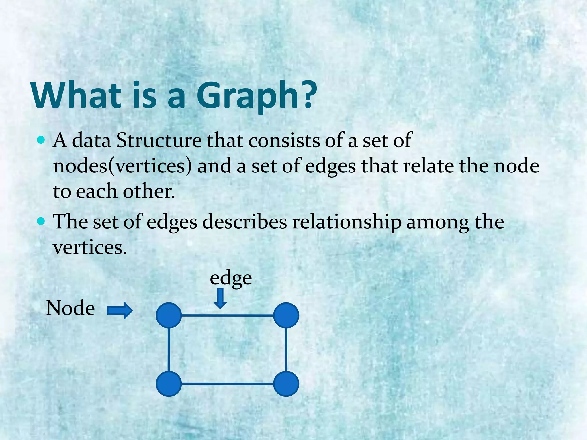
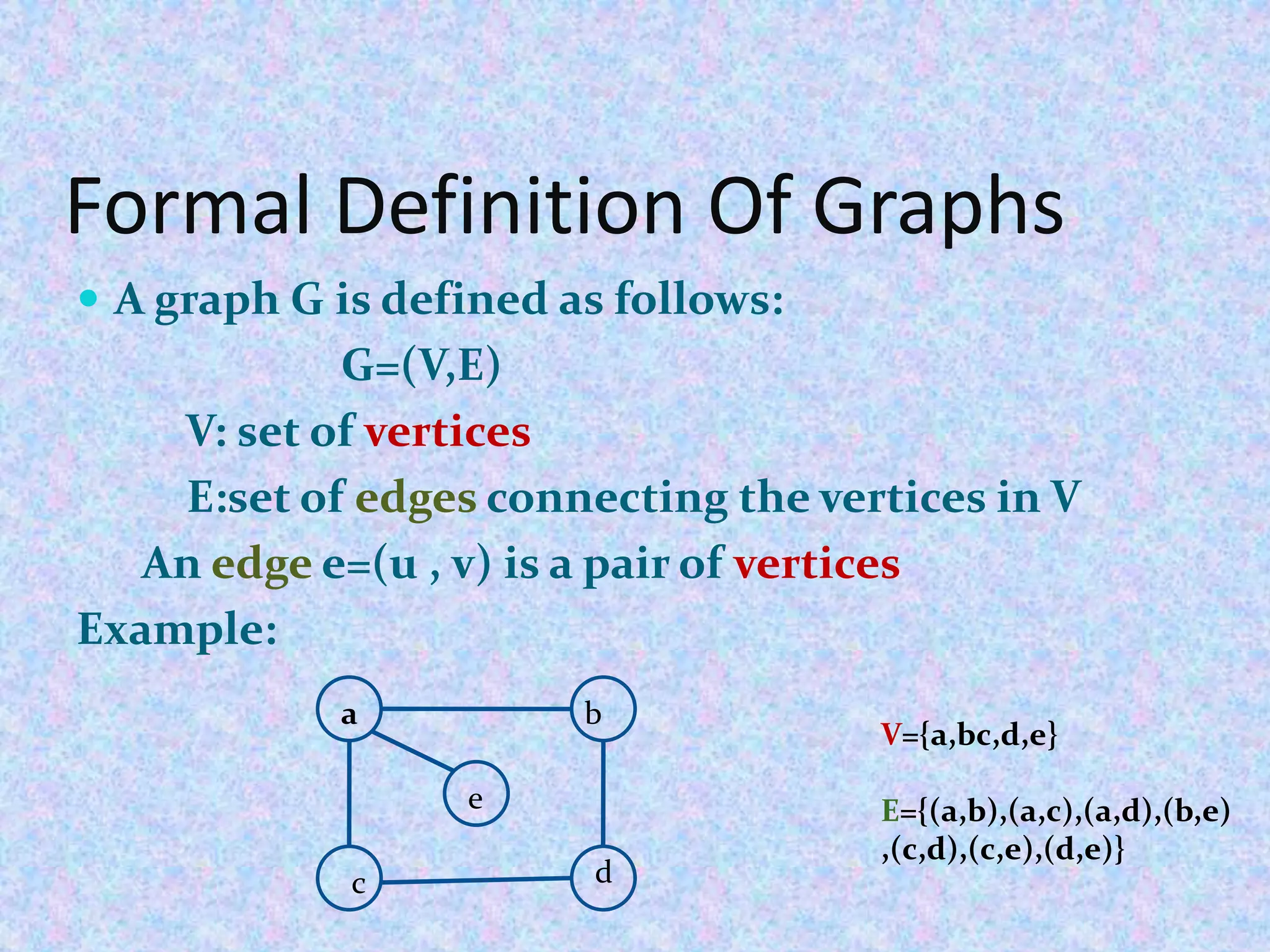
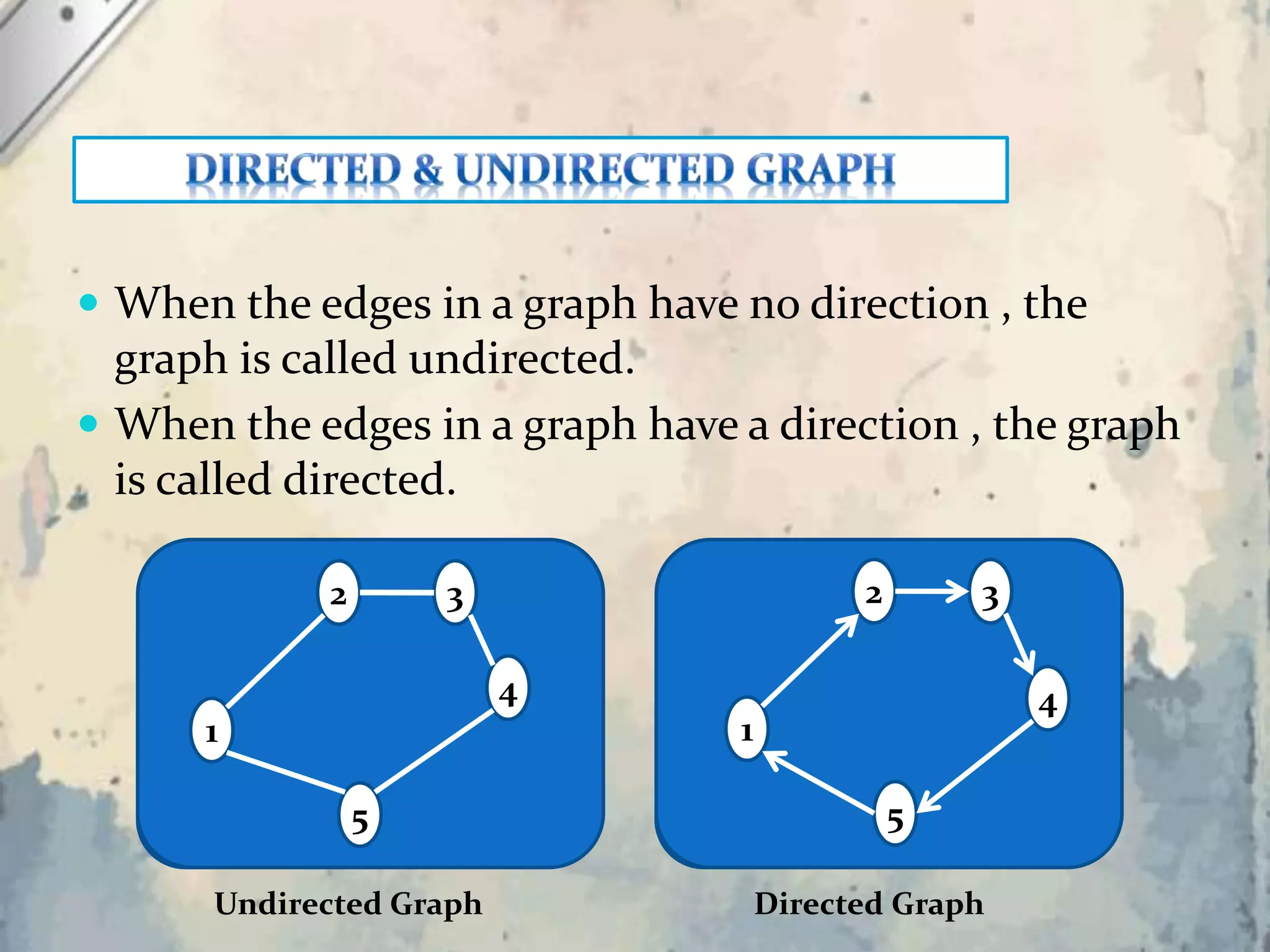
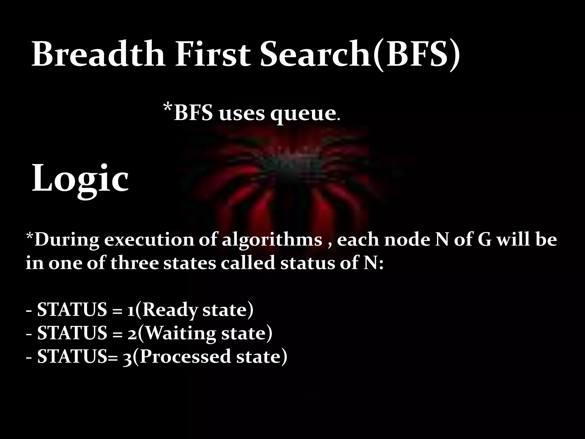
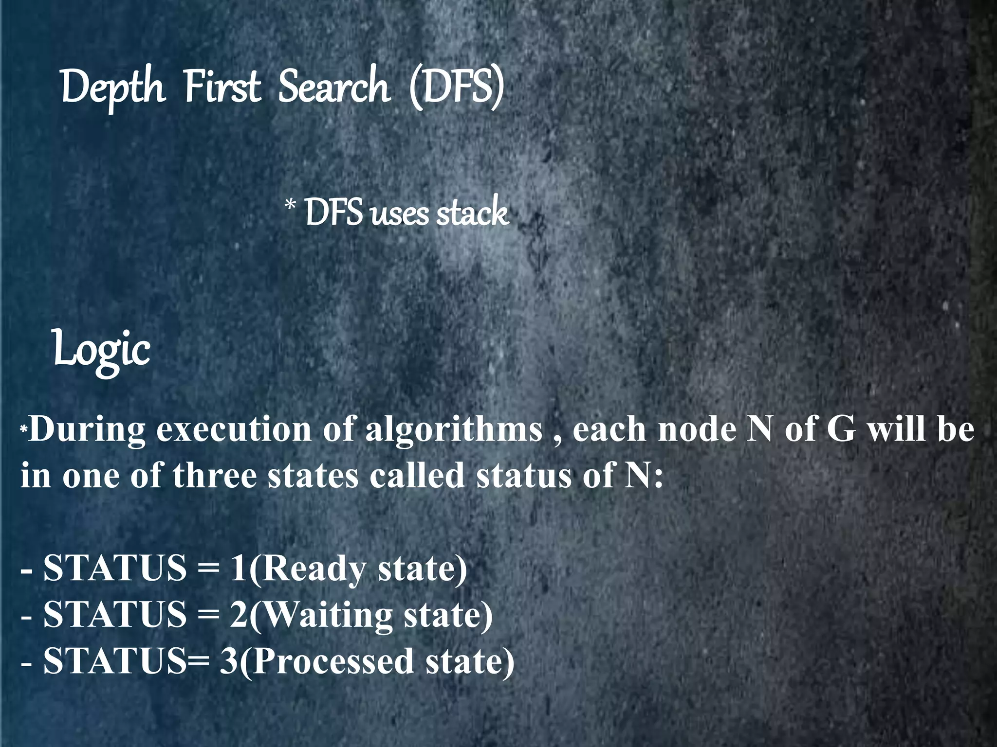
The document explains the concept of graphs as a data structure consisting of vertices and edges, detailing both undirected and directed graphs. It provides formal definitions, examples, and various representations of graphs including adjacency matrices and adjacency lists, along with methods for traversing graphs like breadth-first search (BFS) and depth-first search (DFS). The algorithms for these traversal methods are outlined step by step, emphasizing the states of nodes during processing.

1. Graph

2. What is a Graph?
 A data Structure that consists of a set of
nodes(vertices) and a set of edges that relate the node
to each other.
 The set of edges describes relationship among the
vertices.
edge
Node

3. Formal Definition Of Graphs
 A graph G is defined as follows:
G=(V,E)
V: set of vertices
E:set of edges connecting the vertices in V
An edge e=(u , v) is a pair of vertices
Example:
a b
c d
e
V={a,bc,d,e}
E={(a,b),(a,c),(a,d),(b,e)
,(c,d),(c,e),(d,e)}

4.  When the edges in a graph have no direction , the
graph is called undirected.
 When the edges in a graph have a direction , the graph
is called directed.
Undirected edge Directed edge
a b a b
1
2
5
4
3
1
2
5
4
3
Undirected Graph Directed Graph

5.  Adjacent nodes : two nodes are adjacent if they are
connected by an edge.
 Path : a sequence of vertices that connect two nodes
in a graph
 Simple path : A simple path is a path in which all
vertices , except possibly in the first and last ,are
different.
 Complete Graph: a graph in which every vertex is
directly connected to every other vertex
a b
A is adjacent to b

6.  Adjacency matrix representation.
 Adjacency lists representation.

7. Adjacency matrix
Let G=(V , E) be a graph with n vertices.
The adjacency matrix of G is a two dimensional array n by
n , say A[5][5].
A B
C D
E
(A) 1
(B) 2
(C) 3
(D)4
(E)5
(A)1 (B)2 (C)3 (D)4 (E)5
0 1 1 1 0
01 0 1 0
1 0 0 1 1
1 1 1 0 1
0 0 1 1 0
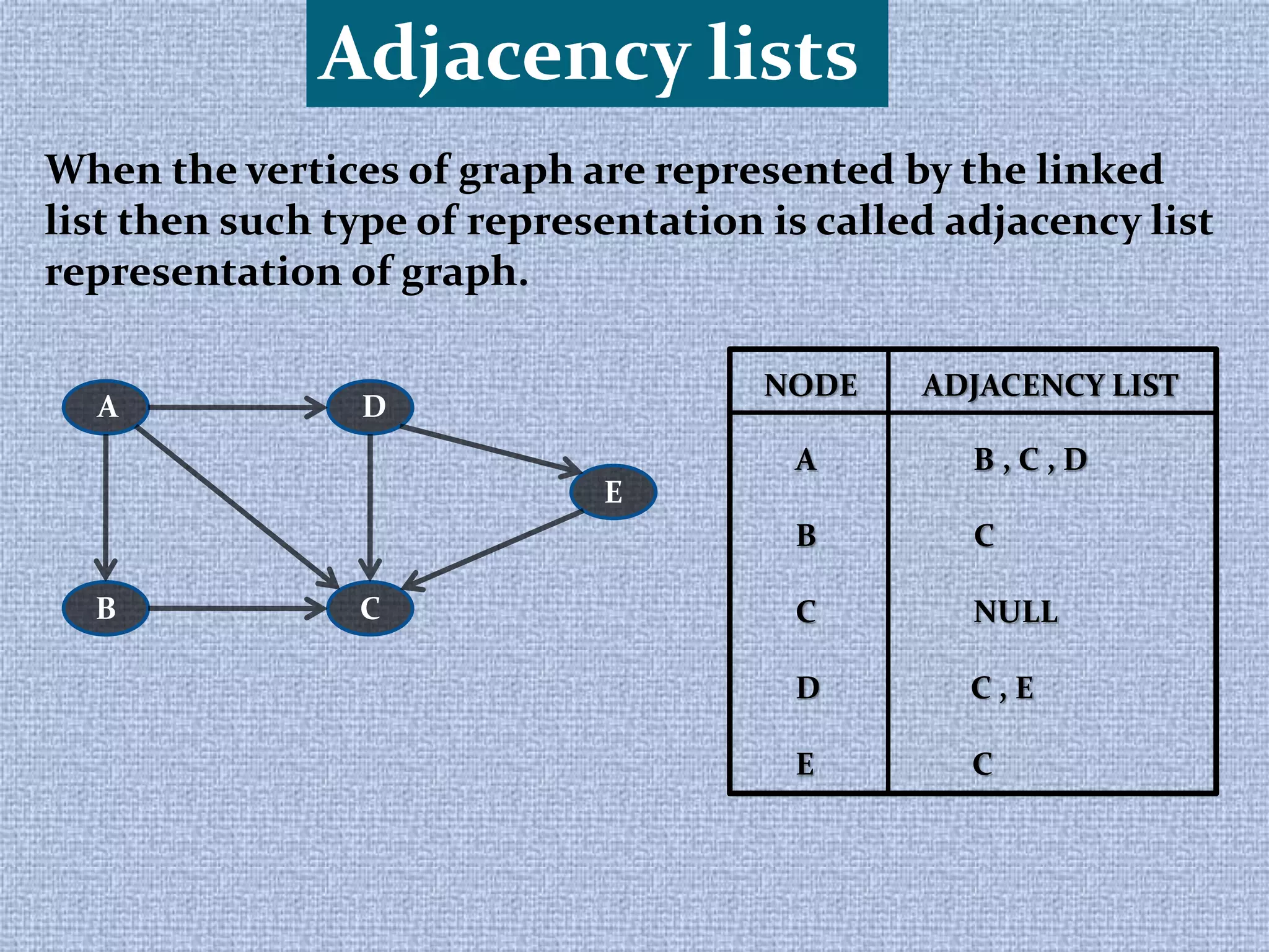
When the adjacent vertices of a graph is represented in the form of matrix
then such type of representation is called Adjacency Matrix
Representation of graph. E.g. A[i][j]
Number of rows = Number of Column
A ij =
O , if Vi is not adjacent to Vj
1 , if Vi , Vj is adjacent

8. Adjacency lists
B C
E
A D
NODE ADJACENCY LIST
A B , C , D
B C
C NULL
D C , E
E C
When the vertices of graph are represented by the linked
list then such type of representation is called adjacency list
representation of graph.

9. Traverse all node in the graph.
Methods
* Breadth – First Search
*Depth - First Search

10. Breadth First Search(BFS)
*BFS uses queue.
Logic
*During execution of algorithms , each node N of G will be
in one of three states called status of N:
- STATUS = 1(Ready state)
- STATUS = 2(Waiting state)
- STATUS= 3(Processed state)

11. ED
C
F
A
B
Algorithm
1.Initialize all nodes to the ready state
(STATUS=1)
2.Put the starting node A in Queue and
change its status to the waiting state
(STATUS=2)
3. [LOOP]
Repeat steps 4 and 5 until queue is empty
4. Remove the front node N of Queue.
Process N and change the status of N to
the processed state (STATUS=3)
5. Add to the rear of queue all the
neighbors of N that are in ready state
(STATUS=1), and change their status to
waiting state (STATUS=2).
[End of Loop]
6. Exit

12. A
ED
CB
F
1.Initialize all nodes to the ready state
(STATUS=1)
1
1
1
1
1
1
2.Put the starting node A in Queue and
change its status to the waiting state
(STATUS=2)
A
2 1.Initialize all nodes to the ready state
(STATUS=1)
2.Put the starting node A in Queue and
change its status to the waiting state
(STATUS=2)
3. [LOOP]
Repeat steps 4 and 5 until queue is
empty
4. Remove the front node N of Queue.
Process N and change the status of N
to the processed state (STATUS=3)
5. Add to the rear of queue all the
neighbors of N that are in ready state
(STATUS=1), and change their status to
waiting state (STATUS=2).
[End of Loop]
6. Exit
3
B C E
2 2
2
D F
3
2
2
3
3
3
3
B
A
C E
D F
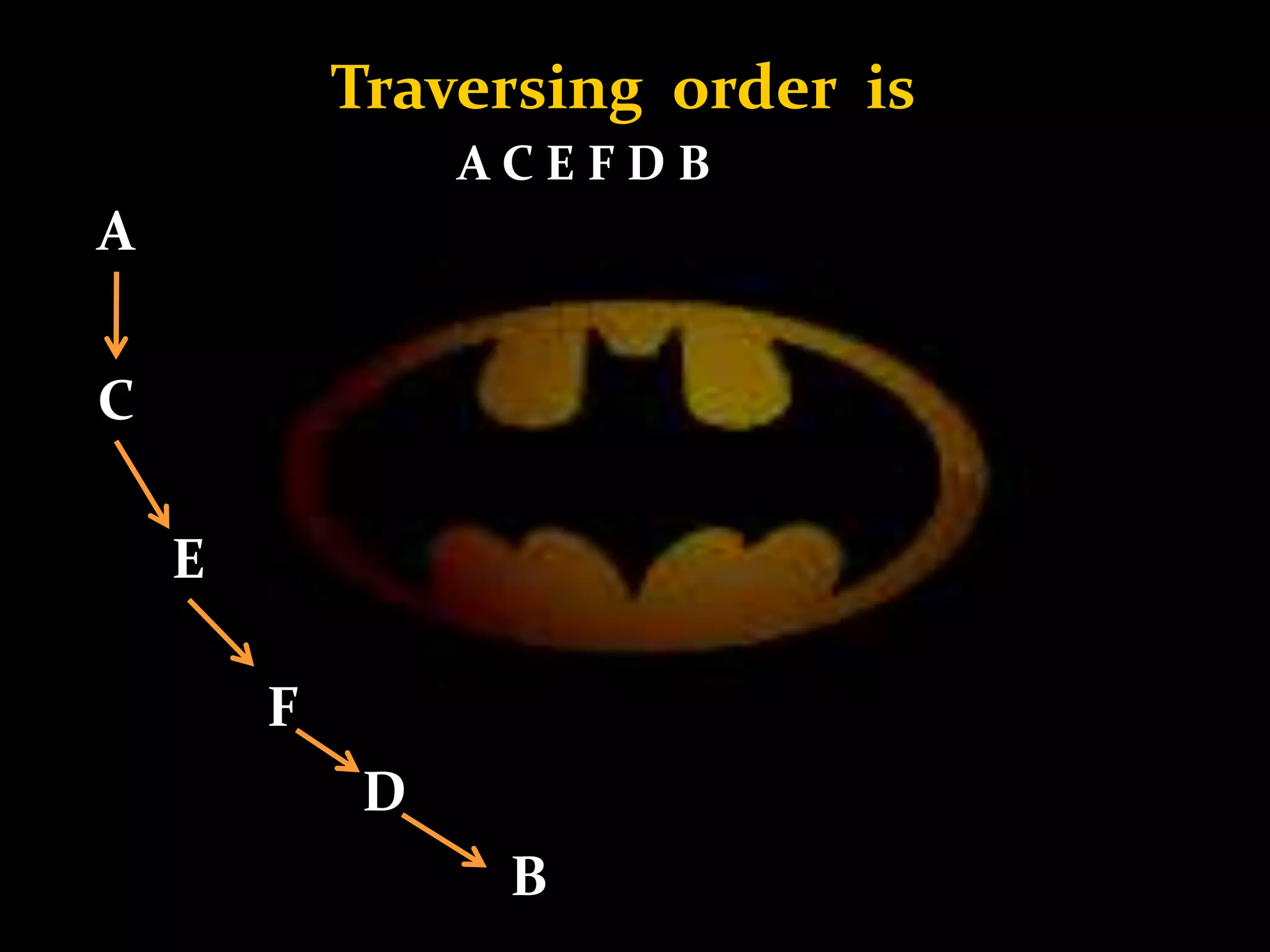
Traversing order – A B C E D F

13. Depth First Search (DFS)
* DFS uses stack
*During execution of algorithms , each node N of G will be
in one of three states called status of N:
- STATUS = 1(Ready state)
- STATUS = 2(Waiting state)
- STATUS= 3(Processed state)
Logic

14. A F
D
C E
B
1.Initialize all nodes to the ready state
(STATUS=1)
2.Push the starting node A onto stack
and change its status to the waiting state
(STATUS=2)
3. [LOOP]
Repeat steps 4 and 5 until stack is
empty
4. Pop the top node N of Stack.
Process N and change the status of N
to the processed state (STATUS=3)
5. Push onto Stack all the neighbors of
N that are still in ready state
(STATUS=1), and change their status to
waiting state (STATUS=2).
[End of Loop]
6. Exit
Algorithm

15. A F
D
C E
B
1.Initialize all nodes to the ready state
(STATUS=1)
1
1
11
1
1
2.Push the starting node A onto stack
and change its status to the waiting state
(STATUS=2)
A
2
A
1.Initialize all nodes to the ready state
(STATUS=1)
2.Push the starting node A onto stack
and change its status to the waiting state
(STATUS=2)
3. [LOOP]
Repeat steps 4 and 5 until stack is
empty
4. Pop the top node N of Stack.
Process N and change the status of N
to the processed state (STATUS=3)
5. Push onto Stack all the neighbors of
N that are still in ready state
(STATUS=1), and change their status to
waiting state (STATUS=2).
[End of Loop]
6. Exit
A
B
C
3
2
2
C
3
D
E
2
2
E
3
F
2
F
3
3 3
D B

16. Traversing order is
A C E F D B
A
C
E
F
D
B

17. Thank you
Jagjot singh chopra
Shivam khanna
2016 csa 1569 2016csa1556