zdcdsc

1. Introduction
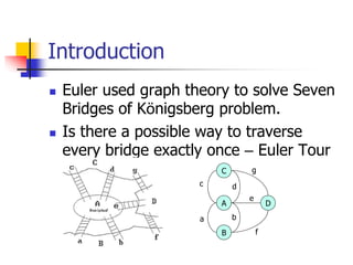
 Euler used graph theory to solve Seven
Bridges of Königsberg problem.
 Is there a possible way to traverse
every bridge exactly once – Euler Tour
C
A
B
D
g
c d
e
b
f
a

2. Definitions
 A graph G=(V,E), V and E are two sets
 V: finite non-empty set of vertices
 E: set of pairs of vertices, edges
 Undirected graph
 The pair of vertices representing any edge is
unordered. Thus, the pairs (u,v) and (v,u)
represent the same edge
 Directed graph
 each edge is represented by a ordered pairs
<u,v>

3. Examples of Graph G1
 G1
 V(G1)={0,1,2,3}
 E(G1)={(0,1),(0,2),
(0,3),(1,2),(1,3),
(2,3)}
0
1 2
3

4. Examples of Graph G2
 G2
 V(G2)={0,1,2,3,4,5,6}
 E(G2)={(0,1),(0,2),
(1,3),(1,4),(2,5),(2,6)}
 G2 is also a tree
 Tree is a special case
of graph
0
1 2
3 4 5 6

5. Examples of Graph G3
 G3
 V(G3)={0,1,2}
 E(G3)={<0,1>,
<1,0>,<1,2>}
 Directed graph
(digraph)
0
1
2

6. Examples of Graphlike Structures
 Graph with self
loops
 Multigraph
0 2
1
2
1
0
3

7. Complete Graph
 A Complete Graph is a graph that has
the maximum number of edges
 For undirected graph with n vertices, the
maximum number of edges is n(n-1)/2
 For directed graph with n vertices, the
maximum number of edges is n(n-1)
 Example: G1

8. Adjacent and Incident
 If (u,v) is an edge in an undirected graph,
 Adjacent: u and v are adjacent
 Incident: The edge (u,v) is incident on
vertices u and v
 If <u,v> is an edge in a directed graph
 Adjacent: u is adjacent to v, and vu is
adjacent from v
 Incident: The edge <u,v> is incident on u
and v

9. Subgraph
 A subgraph of G is a graph G’ such that
 V(G’)  V(G)
 E(G’)  E(G)
 Some of the subgraph of G1
0
0
1 2 3
1 2
0
1 2
3
(i) (ii) (iii) (iv)
G1
0
1 2
3

10. Subgraph
 Some of the subgraphsof G3
0
0
1
0
1
2
0
1
2
(i) (ii) (iii) (iv)
0
1
2
G3

11. Path
 Path from u to v in G
 a sequence of vertices u, i1,
i2,...,ik, v
 If G is undirected: (u,i1), (i1,i2),...,
(ik,v)E(G)
 If G is directed:
<u,i1>,<i1,i2>,...,<ik,v>E(G)
 Length
 The length of a path is the
number of edges on it.
 Length of 0,1,3,2 is 3
0
1 2
3

12. Simple Path
 Simple Path
 is a path in which all
vertices except
possibly the first and
last are distinct.
 0,1,3,2 is simple
path
 0,1,3,1 is path but
not simple
0
1 2
3

13. Cycle
 Cycle
 a simple path, first and
last vertices are same.
 0,1,2,0 is a cycle
 Acyclic graph
 No cycle is in graph
0
1 2
3

14. Connected
 Connected
 Two vertices u and v are
connected if in an
undirected graph G,  a path
in G from u to v.
 A graph G is connected, if
any vertex pair u,v is
connected
 Connected Component
 a maximal connected
subgraph.
 Tree is a connected acyclic
graph
1
2 3
4
connected
connected

15. Strongly Connected
 Strongly Connected
 u, v are strongly
connected if in a
directed graph (digraph)
G,  a path in G from u
to v.
 A directed graph G is
strongly connected, if
any vertex pair u,v is
connected
 Strongly Connected
Component
 a maximal strongly
connected subgraph
1
2
1
2
3
3
G3

16. Degree
 Degree of Vertex
 is the number of edges incident to that
vertex
 Degree in directed graph
 Indegree
 Outdegree
 Summation of all vertices’ degrees are
2|E|

17. Graph Representations
 Adjacency Matrix
 Adjacency Lists
 Adjacency Multilists
 Weighted Edge

18. Graph Representations
undirected graph
degree
0
1 2
3 4 5 6
G1
G2
3
2
3 3
1 1 1 1
directed graph
in-degree
out-degree
0
1
2
in:1, out: 1
in: 1, out: 2
in: 1, out: 0
0
1 2
3
3
3
3

19. Graph Representations
 ADT for Graph
structure Graph is
objects: a nonempty set of vertices and a set of undirected edges, where
each edge is a pair of vertices
functions: for all graph  Graph, v, v1 and v2  Vertices
Graph Create()::=return an empty graph
Graph InsertVertex(graph, v)::= return a graph with v inserted. v has no
incident edge.
Graph InsertEdge(graph, v1,v2)::= return a graph with new edge
between v1 and v2
Graph DeleteVertex(graph, v)::= return a graph in which v and all edges
incident to it are removed
Graph DeleteEdge(graph, v1, v2)::=return a graph in which the edge (v1,
v2)
is removed
Boolean IsEmpty(graph)::= if (graph==empty graph) return TRUE
else return FALSE
List Adjacent(graph,v)::= return a list of all vertices that are adjacent to
v

20. Graph Representations
 Adjacency Matrix
 Adjacency Lists
 Adjacency Multilists

21. Adjacency Matrix
 Adjacency Matrix : let G = (V, E) with n
vertices, n  1. The adjacency matrix of G is a
2-dimensional n  n matrix, A
 A(i, j) = 1 iff (vi, vj) E(G)
(vi, vj for a diagraph)
 A(i, j) = 0 otherwise.
 The adjacency matrix for an undirected graph
is symmetric; the adjacency matrix for a
digraph need not be symmetric

22. Example
0
1
1
1
1
0
1
1
1
1
0
1
1
1
1
0












0
1
0
1
0
0
0
1
0










0
1
1
0
0
0
0
0
1
0
0
1
0
0
0
0
1
0
0
1
0
0
0
0
0
1
1
0
0
0
0
0
0
0
0
0
0
1
0
0
0
0
0
0
1
0
1
0
0
0
0
0
0
1
0
1
0
0
0
0
0
0
1
0


























G1
G2
G4
0
1 2
3
0
1
2
1
0
2
3
4
5
6
7
symmetric
undirected: n2/2
directed: n2

23. Merits of Adjacency Matrix
 From the adjacency matrix, to determine
the connection of vertices is easy
 The degree of a vertex is
 For a digraph, the row sum is the
out_degree, while the column sum is the
in_degree
ind vi A j i
j
n
( ) [ , ]




0
1
outd vi A i j
j
n
( ) [ , ]




0
1
adj mat i j
j
n
_ [ ][ ]



0
1

24. Adjacency Lists
 Replace n rows of the adjacency matrix
with n linked list

25. Data Structures for Adjacency
Lists
#define MAX_VERTICES 50
typedef struct node *node_pointer;
typedef struct node {
int vertex;
struct node *link;
};
node_pointer graph[MAX_VERTICES];
int n=0; /* vertices currently in use */
Each row in adjacency matrix is represented as an adjacency list.

26. Example(1)
0
1
2
3
0
1
2
1 2 3
0 2 3
0 1 3
0 1 2
G1
1
0 2
G3
0
1 2
3
0
1
2

27. Example(2)
0
1
2
3
4
5
6
7
1 2
0 3
0 3
1 2
5
4 6
5 7
6
G4
1
0
2
3
4
5
6
7
An undirected graph with n vertices and e edges ==> n head nodes and 2e list nodes

28. Interesting Operations
degree of a vertex in an undirected graph
–# of nodes in adjacency list
# of edges in a graph
–determined in O(n+e)
out-degree of a vertex in a directed graph
–# of nodes in its adjacency list
in-degree of a vertex in a directed graph
–traverse the whole data structure

29. Compact Representation
1
0
2
3
4
5
6
7
node[0] … node[n-1]: starting point for vertices
node[n]: n+2e+1
node[n+1] … node[n+2e]: head node of edge
[0] 9 [8] 23 [16] 2
[1] 11 [9] 1 [17] 5
[2] 13 [10] 2 [18] 4
[3] 15 [11] 0 [19] 6
[4] 17 [12] 3 [20] 5
[5] 18 [13] 0 [21] 7
[6] 20 [14] 3 [22] 6
[7] 22 [15] 1
0
1
2
3
4
5
6
7

30. Figure 6.10: Inverse adjacency list for G3



0
1
2
1 NULL
0 NULL
1 NULL
0
1
2
Determine in-degree of a vertex in a fast way.

31. Figure 6.11: Alternate node structure for
adjacency lists (p.267)
tail head column link for head row link for tail

32. Figure 6.12: Orthogonal representation for
graph G3(p.268)
0 1 2
2 NULL
1
0
1 0NULL
0 1 NULL NULL
1 2 NULL NULL
0
1
2
0
1
0
1
0
0
0
1
0











33. Figure 6.13:Alternate order adjacency list for
G1 (p.268)
 3  2 NULL
1 
0
 2  3 NULL
0 
1
 3  1 NULL
0 
2
 2  0 NULL
1 
3
headnodes vertax link
Order is of no significance.
0
1 2
3

34. Adjacency Multilists
 An edge in an undirected graph is represented
by two nodes in adjacency list representation.
 Adjacency Multilists
 lists in which nodes may be shared among several
lists.
(an edge is shared by two different paths)
marked vertex1 vertex2 path1 path2

35. Example for Adjacency
Multlists
0 1 N2 N4
0 2 N3 N4
0 3 N5
1 2 N5 N6
1 3 N6
2 3
N1
N2
N3
N4
N5
N6
0
1
2
3
edge (0,1)
edge (0,2)
edge (0,3)
edge (1,2)
edge (1,3)
edge (2,3)
(1,0)
(2,0)
(3,0)
(2,1)
(3,1)
(3,2)
0
1 2
3
six edges
Lists: vertex 0: M1->M2->M3, vertex 1: M1->M4->M5
vertex 2: M2->M4->M6, vertex 3: M3->M5->M6

36. Data Structures for Adjacency
Multilists
typedef struct edge *edge_pointer;
typedef struct edge {
short int marked;
int vertex1, vertex2;
edge_pointer path1, path2;
};
edge_pointer graph[MAX_VERTICES];
marked vertex1 vertex2 path1 path2

37. Some Graph Operations
 Traversal
Given G=(V,E) and vertex v, find all wV,
such that w connects v.
 Depth First Search (DFS)
preorder tree traversal
 Breadth First Search (BFS)
level order tree traversal
 Connected Components
 Spanning Trees

38. *Figure 6.19:Graph G and its adjacency
lists (p.274)
depth first search: v0, v1, v3, v7, v4, v5, v2, v6
breadth first search: v0, v1, v2, v3, v4, v5, v6, v7

39. Weighted Edge
 In many applications, the edges of a
graph are assigned weights
 These weights may represent the
distance from one vertex to another
 A graph with weighted edges is called a
network

40. Elementary Graph Operations
 Traversal: given G = (V,E) and vertex v,
find or visit all wV, such that w connects v
 Depth First Search (DFS)
 Breadth First Search (BFS)
 Applications
 Connected component
 Spanning trees
 Biconnected component

41. Depth First Search
 Begin the search by visiting the start
vertex v
 If v has an unvisited neighbor, traverse it
recursively
 Otherwise, backtrack
 Time complexity
 Adjacency list: O(|E|)
 Adjacency matrix: O(|V|2)

42. Example
 Start vertex: 0
 Traverse order: 0, 1, 3, 7, 4, 5, 2, 6
0
1 2
3 4 5 6
7

43. Depth First Search
#define FALSE 0
#define TRUE 1
short int visited[MAX_VERTICES];
void dfs(int v)
{
node_pointer w;
visited[v]= TRUE;
printf(“%5d”, v);
for (w=graph[v]; w; w=w->link)
if (!visited[w->vertex])
dfs(w->vertex);
}
Data structure
adjacency list: O(e)
adjacency matrix: O(n2)

44. Breadth First Search
 Begin the search by visiting the start
vertex v
 Traverse v’s neighbors
 Traverse v’s neighbors’ neighbors
 Time complexity
 Adjacency list: O(|E|)
 Adjacency matrix: O(|V|2)

45. Example
 Start vertex: 0
 Traverse order: 0, 1, 2, 3, 4, 5, 6, 7
0
1 2
3 4 5 6
7

46. Breadth First Search
typedef struct queue *queue_pointer;
typedef struct queue {
int vertex;
queue_pointer link;
};
void addq(queue_pointer *,
queue_pointer *, int);
int deleteq(queue_pointer *);

47. Breadth First Search (Continued)
void bfs(int v)
{
node_pointer w;
queue_pointer front, rear;
front = rear = NULL;
printf(“%5d”, v);
visited[v] = TRUE;
addq(&front, &rear, v);

48. Breadth First Search (Continued)
while (front) {
v= deleteq(&front);
for (w=graph[v]; w; w=w->link)
if (!visited[w->vertex]) {
printf(“%5d”, w->vertex);
addq(&front, &rear, w-
>vertex);
visited[w->vertex] = TRUE;
}
}
}

49. Connected Component
 Find all connected component in a
graph G
 Select one unvisited vertex v, and start
DFS (or BFS) on v
 Select one another unvisited vertex v,
and start DFS (or BFS) on v

50. Example
 Start on 0
 0, 1, 3, 4, 7 is visited
 These 5 vertices is in the
same connected
component
 Choose 2
 2, 5, 6 is visited
0
1 2
3 4 5 6
7

51. Connected Component
void connected(void)
{
for (i=0; i<n; i++) {
if (!visited[i]) {
dfs(i);
printf(“n”);
}
}
}

52. Other Applications
 Find articulation point (cut vertex) in undirected connected
graph
 Find bridge (cut edge) in undirected connected graph
 Find strongly connected component in digraph
 Find biconnected connected component in connected
graph
 Find Euler path in undirected connected graph
 Determine whether a graph G is bipartite graph?
 Determine whether a graph G contain cycle?
 Calculate the radius and diameter of a tree

53. Spanning Trees
 Spanning tree: any tree consisting only
edges in G and including all vertices in
G is called.
 Example:
 How many spanning trees?

54. Example

55. Spanning Trees
 Either dfs or bfs can be used to create a
spanning tree
 When dfs is used, the resulting spanning tree is
known as a depth first spanning tree
 When bfs is used, the resulting spanning tree is
known as a breadth first spanning tree
 While adding a nontree edge into any
spanning
tree, this will create a cycle

56. DFS VS BFS Spanning Tree
0
1 2
3 4 5 6
7
0
1 2
3 4 5 6
7
DFS Spanning BFS Spanning
0
1 2
3 4 5 6
7 nontree edge
cycle

57. Spanning Trees
 A spanning tree is a minimal subgraph, G’, of G
 such that V(G’)=V(G) and G’ is connected.
 Any connected graph with n vertices must have
at least n-1 edges.
 A biconnected graph is a connected graph that has
 no articulation points.
0
1 2
3 4 5 6
7
biconnected graph

58. Spanning Trees
connected graph
1
3 5
6
8 9
0
2
4
2
1
3 5
6
8 9
0
7
2
4
two connected components
2
1
3 5
6
0 8 9
7
4
one connected graph
7

59. Spanning Trees
1
3 5
6
0 8 9
7
2
4
1
0
1
3
2
4
3 5
8
7
9
7
5
6
7
biconnected components
biconnected component: a maximal connected subgraph H
(no subgraph that is both biconnected and properly contains H)

60. Spanning Trees
8
0
1
2
4
5
6
4
3
0 5
9 8 9 8
7 7
3
4 5
7
6
9 8
2
0
1
0
6
1
3
(a) depth first spanning tree (b)
2 5
dfn
depth
first
number
nontree
edge
(back edge)
nontree
edge
(back edge)
Why is cross edge impossible?
If u is an ancestor of v then dfn(u) < dfn(v).
1 6
2
4
7
9
5
Find biconnected component of a connected undirected
graphby depth first spanning tree

61. *Figure 6.24: dfn and low values for dfs
spanning tree with root =3(p.281)
Vertax 0 1 2 3 4 5 6 7 8 9
dfn 4 3 2 0 1 5 6 7 9 8
low 4 0 0 0 0 5 5 5 9 8

62. Spanning Trees
8 9
3
4 5
7
6
9 8
2
0
1
6
7
1 5
2
4
3
low(u)=min{dfn(u),
min{low(w)|w is a child of u},
min{dfn(w)|(u,w) is a back edge}
u: articulation point
low(child)  dfn(u)
*The root of a depth first spanning
tree is an articulation point iff
it has at least two children.
*Any other vertex u is an articulation
point iff it has at least one child w
such that we cannot reach an ancestor
of u using a path that consists of
(1) only w (2) descendants of w (3)
single back edge.

63. Spanning Trees
8 9
3
4 5
7
6
9 8
2
0
1
6
7
1
5
2
4
3
vertex dfn low child low_child low:dfn
0 4 4 (4,n,n) null null null:4
1 3 0 (3,4,0) 0 4 4  3 
2 2 0 (2,0,n) 1 0 0 < 2
3 0 0 (0,0,n) 4,5 0,5 0,5  0 
4 1 0 (1,0,n) 2 0 0 < 1
5 5 5 (5,5,n) 6 5 5  5 
6 6 5 (6,5,n) 7 5 5 < 6
7 7 5 (7,8,5) 8,9 9,8 9,8  7 
8 9 9 (9,n,n) null null null, 9
9 8 8 (8,n,n) null null null, 8

64. *Program 6.5: Initializaiton of dfn and low
(p.282)
 void init(void)
{
int i;
for (i = 0; i < n; i++) {
visited[i] = FALSE;
dfn[i] = low[i] = -1;
}
num = 0;
}

65. *Program 6.4: Determining dfn and low
(p.282)
void dfnlow(int u, int v)
{
node_pointer ptr;
int w;
dfn[u] = low[u] = num++;
for (ptr = graph[u]; ptr; ptr = ptr ->link) {
w = ptr ->vertex;
if (dfn[w] < 0) {
/*w is an unvisited vertex */
dfnlow(w, u);
low[u] = MIN2(low[u], low[w]);
}
else if (w != v)
low[u] =MIN2(low[u], dfn[w] ); }}

66. *Program 6.6: Biconnected components of a
graph (p.283)
void bicon(int u, int v)
{
node_pointer ptr;
int w, x, y;
dfn[u] = low[u] = num ++;
for (ptr = graph[u]; ptr; ptr = ptr->link)
{
w = ptr ->vertex;
if ( v != w && dfn[w] < dfn[u] )
add(&top, u, w);
if(dfn[w] < 0) {
bicon(w, u);
low[u] = MIN2(low[u], low[w]);

67. *Program 6.6: Biconnected components of a
graph (p.283) (con.)
if (low[w] >= dfn[u] ){ articulation point
printf(“New biconnected component: “);
do { /* delete edge from stack */
delete(&top, &x, &y);
printf(“ <%d, %d>” , x, y);
} while (!(( x = = u) && (y = = w)));
printf(“n”);
}
}
else if (w != v) low[u] = MIN2(low[u], dfn[w]);}}

68. Minimum Cost Spanning Tree
 The cost of a spanning tree of a weighted
undirected graph is the sum of the costs of
the edges in the spanning tree
 A minimum cost spanning tree is a spanning
tree of least cost
 Three different algorithms can be used
 Kruskal
 Prim
 Sollin
Select n-1 edges from a weighted graph
of n vertices with minimum cost.

69. Greedy Strategy
 An optimal solution is constructed in stages
 At each stage, the best decision is made at
this time
 Since this decision cannot be changed later,
we make sure that the decision will result in a
feasible solution
 Typically, the selection of an item at each
stage is based on a least cost or a highest
profit criterion

70. Kruskal’s algorithm for
finding MST
Step 1: Sort all edges into nondecreasing order.
Step 2: Add the next smallest weight edge to the
forest if it will not cause a cycle.
Step 3: Stop if n-1 edges. Otherwise, go to Step2.
Time complexity: O(|E| log |E|)

71. Example

72. Kruskal’s Algorithm
T= {};
while (T contains less than n-1 edges
&& E is not empty) {
choose a least cost edge (v,w) from E;
delete (v,w) from E;
if ((v,w) does not create a cycle in T)
add (v,w) to T
else discard (v,w);
}
if (T contains fewer than n-1 edges)
printf(“No spanning treen”);

73. Prim’s Algorithm
Step 1: x  V, Let A = {x}, B = V - {x}.
Step 2: Select (u, v)  E, u  A, v  B such
that (u, v) has the smallest weight between A
and B.
Step 3: Put (u, v) in the tree. A = A  {v}, B =
B - {v}
Step 4: If B = , stop; otherwise, go to Step 2.
 Time complexity : O(|V|2)

74. Example

75. Prim’s Algorithm
T={};
TV={0};
while (T contains fewer than n-1 edges)
{
let (u,v) be a least cost edge such
that and
if (there is no such edge ) break;
add v to TV;
add (u,v) to T;
}
if (T contains fewer than n-1 edges)
printf(“No spanning treen”);
u TV
 v TV


76. Sollin’s Algorithm
0
1
2
3
4
5 6
28
16
12
18
24
22
25
10
14
vertex edge
0 0 -- 10 --> 5, 0 -- 28 --> 1
1 1 -- 14 --> 6, 1-- 16 --> 2, 1 -- 28 --> 0
2 2 -- 12 --> 3, 2 -- 16 --> 1
3 3 -- 12 --> 2, 3 -- 18 --> 6, 3 -- 22 --> 4
4 4 -- 22 --> 3, 4 -- 24 --> 6, 5 -- 25 --> 5
5 5 -- 10 --> 0, 5 -- 25 --> 4
6 6 -- 14 --> 1, 6 -- 18 --> 3, 6 -- 24 --> 4

77. Sollin’s Algorithm (con.)
0
1
2
3
4
5 6
10
0
22
12
16
14
0
1
2
3
4
5 6
10
22
12
14
0
1
2
3
4
5 6
{0,5}
5 4 0 1
25 28
{1,6}
1 2
16 28
1
6 3 6 4
18 24

78. Shortest Paths
 Given a directed graph G=(V,E), a
weighted function, w(e).
 How to find the shortest path from u to
v?

79. Example:
*Figure 6.29: Graph and shortest paths from v0 (p.293)
 shortest paths from v0 to all destinations

80. Shortest Paths
 Single source all destinations:
 Nonnegative edge costs: Dijkstra’s
algorithm
 General weights: Bellman-Ford’s algorithm
 All pairs shortest path
 Floyd’s algorithm

81. Single Source All Destinations:
Nonnegative Edge Costs
 Given a directed graph G=(V,E), a
weighted function, w(e), and a source
vertex v0
 We wish to determine a shortest path
from v0 to each of the remaining
vertices of G

82. Dijkstra’s algorithm
 Let S denotes the set of vertices, including v0,
whose shortest paths have been found.
 For w not in S, let distance[w] be the length
of the shortest path starting from v0, going
through vertices only in S, and ending in w.
 We can find a vertex u not in S and
distance[u] is minimum, and add u into S.
 Maintain distance properly
 Complexity: (|V|2)

83. Dijkstra’s algorithm
1 2 3 4 5 6 7 8
1 0
2 300 0
3 1000 800 0
4 1200 0
5 1500 0 250
6 1000 0 900 1400
7 0 1000
8 1700 0
Cost adjacency matrix.
All entries not shown
are +.

84. Vertex
Iteration S Selected (1) (2) (3) (4) (5) (6) (7) (8)
Initial ----
1 5 6 + + + 1500 0 250 + +
2 5,6 7 + + + 1250 0 250 1150 1650
3 5,6,7 4 + + + 1250 0 250 1150 1650
4 5,6,7,4 8 + + 2450 1250 0 250 1150 1650
5 5,6,7,4,8 3 3350 + 2450 1250 0 250 1150 1650
6 5,6,7,4,8,3 2 3350 3250 2450 1250 0 250 1150 1650
5,6,7,4,8,3,2 3350 3250 2450 1250 0 250 1150 1650

85. All Pairs Shortest Paths
 Given a directed graph G=(V,E), a
weighted function, w(e).
 How to find every shortest path from u
to v for all u,v in V?

86. Floyd’s Algorithm
 Represent the graph G by its length
adjacency matrix with length[i][j]
 If the edge <i, j> is not in G, the Represent
the graph G by its length adjacency matrix
with length[i][j] is set to some sufficiently
large number
 Ak[i][j] is the Represent the graph G by its
length adjacency matrix with length of the
shortest path form i to j, using only those
intermediate vertices with an index  k
 Complexity: O(|V|3)

87. Ak[i][j]
 A-1[i][j] = length[i][j]
 Ak[i][j] = the length (or cost) of the
shortest path from i to j going through
no intermediate vertex of index greater
than k
= min{ Ak-1[i][j], Ak-1[i][k]+Ak-1[k][j] }
k≧0

88. Example
v0
v2
v1
6
2
3
11
4
0 1 2
0 0 4 11
1 6 0 2
2 3  0
A-1
0 1 2
0 0 4 11
1 6 0 2
2 3 7 0
A0
v0
v2
v1
6
2
3
11
4

89. Example cont.
0 1 2
0 0 4 6
1 6 0 2
2 3 7 0
A1
v0
v2
v1
6
2
3
11
4
0 1 2
0 0 4 6
1 5 0 2
2 3 7 0
A2
v0
v2
v1
6
2
3
11
4

90. Activity Networks
 We can divide all but simplest projects
into several subprojects called activity.
 Model it as a graph
 Activity-on-Vertex (AOV) Networks
 Activity-on-Edge (AOE) Networks

91. Activity on Vertex (AOV)
Networks
 An activity on vertex, or AOV network,
is a directed graph G in which the
vertices represent tasks or activities and
the edges represent the precedence
relation between tasks

92. Example
 C3 is C1’s successor
 C1 is C3’s predecessor
C1
C2
C3
C4 C5 C6
C7
C8
C9
C10 C11
C12
C14
C13
C15

93. Topological Ordering
 A topological order is a linear ordering
of the vertices of a graph such that, for
any two vertices, i, j, if i is a
predecessor of j in the network then I
precedes j in the ordering

94. Example
 C1 C2 C4 C5 C3 C6 C8 C7 C10 C13 C12
C14 C15 C11 C9
 May not unique
C1
C2
C3
C4 C5 C6
C7
C8
C9
C10 C11
C12
C14
C13
C15

95. Topological Sort
 Find a vertex v such that v has no
predecessor, output it. Then delete it
from network
 Repeat this step until all vertices are
deleted
 Time complexity: O(|V| + |E|)

96. Example
 v0 has no predecessor, output it. Then
delete it and three edges
v0
v1
v2
v3
v4
v5
v0
v1
v2
v3
v4
v5

97. Example cont.
 Choose v3, output it
 Final result: v0, v3, v2, v1, v4, v5
v1
v2
v3
v4
v5

98. *Program 6.13: Topological sort (p.306)
for (i = 0; i <n; i++) {
if every vertex has a predecessor {
fprintf(stderr, “Network has a cycle.n “ );
exit(1);
}
pick a vertex v that has no predecessors;
output v;
delete v and all edges leading out of v
from the network;
}

99. Issues in Data Structure
Consideration
 Decide whether a vertex has any
predecessors.
 Each vertex has a count.
 Decide a vertex together with all its
incident edges.
 Adjacency list

100. *Figure 6.40:Adjacency list representation of
Figure 6.30(a)(p.309)
0  1  2  3 NULL
1  4 NULL
1  4  5 NULL
1  5  4 NULL
3 NULL
2 NULL
V0
V1
V2
V3
V4
V5
v0
v1
v2
v3
v4
v5
count link
headnodes
vertex link
node

101. *(p.307)
 typedef struct node *node_pointer;
typedef struct node {
int vertex;
node_pointer link;
};
typedef struct {
int count;
node_pointer link;
} hdnodes;
hdnodes graph[MAX_VERTICES];

102. *Program 6.14: Topological sort (p.308)
 void topsort (hdnodes graph [] , int n)
{
int i, j, k, top;
node_pointer ptr;
/* create a stack of vertices with no predecessors
*/
top = -1;
for (i = 0; i < n; i++)
if (!graph[i].count) {
graph[i].count = top; top = i;
}
for (i = 0; i < n; i++)
if (top == -1) {
fprintf(stderr, “n Network has a cycle. Sort
terminated. n”);
exit(1);
}

103. *Program 6.14: Topological sort (p.308) (con.)
else {
j = top; /* unstack a vertex */
top = graph[top].count;
printf(“v%d, “, j);
for (ptr = graph [j]. link; ptr ;ptr = ptr ->link )
{
/*decrease the count of the successor vertices of j*/
k = ptr ->vertex;
graph[k].count --;
if (!graph[k].count) {
/* add vertex k to the stack*/
graph[k].count = top;
top = k;
}
}
}
}

104. Activity on Edge (AOE) Networks
 Activity on edge or AOE, network is an activity
network closely related to the AOV network. The
directed edges in the graph represent tasks or
activities to be performed on a project.
 directed edge
 tasks or activities to be performed
 vertex
 events which signal the completion of certain activities
 number
 time required to perform the activity

105. Example: *Figure 6.41:An AOE network(p.310)
 Activities: a0, a1,…
 Events :v0,v1,…
V0
V1
V2
V3
V4
V6
V7
V8
V5
finish
a0 = 6
start
a1 = 4
a2 = 5
a4 = 1
a3 = 1
a5 = 2
a6 = 9
a7 = 7
a8 = 4
a10 = 4
a9 = 2

106. Application of AOE Network
 Evaluate performance
 minimum amount of time
 activity whose duration time should be shortened
 …
 Critical path
 a path that has the longest length
 minimum time required to complete the project
 v0, v1, v4, v7, v8 or v0, v1, v4, v6, v8 (18)

107. Critical Path
 A critical path is a path that has the
longest length. (v0, v1, v4, v7, v8)
V0
V1
V2
V3
V4
V6
V7
V8
V5
a0 = 6
a1 = 4
a2 = 5
a4 = 1
a3 = 1
a5 = 2
a6 = 9
a7 = 7
a8 = 4
a10 = 4
a9 = 2
start finish
6 + 1 + 7 + 4 = 18 (Max)

108. Earliest Time
 The earliest time of an activity, ai, can occur is the length
of the longest path from the start vertex v0 to ai’s start
vertex.
（Ex: the earliest time of activity a7 can occur is 7.）
 We denote this time as early(i) for activity ai.
∴ early(6) = early(7) = 7.
V0
V1
V2
V3
V4
V6
V7
V8
V5
finish
a0 = 6
start
a1 = 4
a2 = 5
a4 = 1
a3 = 1
a5 = 2
a6 = 9
a7 = 7
a8 = 4
a10 = 4
a9 = 2
6/?
0/?
7/? 16/?
0/?
5/?
7/?
14/?
7/?
4/?
0/?
18

109. Latest Time
 The latest time, late(i), of activity, ai, is defined to be the
latest time the activity may start without increasing the
project duration.
 Ex: early(5) = 5 & late(5) = 8; early(7) = 7 & late(7) = 7
V0
V1
V2
V3
V4
V6
V7
V8
V5
finish
a0 = 6
start
a1 = 4
a2 = 5
a4 = 1
a3 = 1
a5 = 2
a6 = 9
a7 = 7
a8 = 4
a10 = 4
a9 = 2
late(5) = 18 – 4 – 4 - 2 = 8
late(7) = 18 – 4 – 7 = 7
6/6
0/1
7/7 16/16
0/3
5/8
7/10
14/14
7/7
4/5
0/0

110. Critical Activity
 A critical activity is an activity for which
early(i) = late(i).
 The difference between late(i) and early(i) is
a measure of how critical an activity is.
Calculation
of
Latest Times
Calculation
of
Earliest Times
Finding
Critical path(s)
To solve
AOE Problem

111. Calculation of Earliest Times
 Let activity ai is represented by edge (u, v).
 early (i) = earliest [u]
 late (i) = latest [v] – duration of activity ai
 We compute the times in two stages:
a forward stage and a backward stage.
 The forward stage:
 Step 1: earliest [0] = 0
 Step 2: earliest [j] = max {earliest [i] + duration of (i, j)}
i is in P(j)
P(j) is the set of immediate predecessors of j.
vu vv
ai

112. *Figure 6.42:Computing earliest from
topological sort (p.313)
V0
V1
V2
V3
V4
V6
V7
V8
V5
4
5
1
1
2
9
7
4
4
2
6

113.  The backward stage:
 Step 1: latest[n-1] = earliest[n-1]
 Step 2: latest [j] = min {latest [i] - duration of (j, i)}
i is in S(j)
S(j) is the set of vertices adjacent from vertex j.
latest[8] = earliest[8] = 18
latest[6] = min{earliest[8] - 2} = 16
latest[7] = min{earliest[8] - 4} = 14
latest[4] = min{earliest[6] – 9; earliest[7] – 7} = 7
latest[1] = min{earliest[4] - 1} = 6
latest[2] = min{earliest[4] - 1} = 6
latest[5] = min{earliest[7] - 4} = 10
latest[3] = min{earliest[5] - 2} = 8
latest[0] = min{earliest[1] – 6; earliest[2] – 4; earliest[3] – 5} = 0
Calculation of Latest Times

114. *Figure 6.43: Computing latest for AOE network of Figure
6.41(a)(p.314)

115. Graph with non-critical activities deleted
V0
V1
V2
V3
V4
V6
V7
V8
V5
finish
a0
start
a1
a2
a4
a3
a5
a6
a7
a8
a10
a9
V0
V1
V4
V6
V7
V8 finish
a0
start
a3 a6
a7 a10
a9
Activity Early Late L - E Critical
a0 0 0 0 Yes
a1 0 2 2 No
a2 0 3 3 No
a3 6 6 0 Yes
a4 4 6 2 No
a5 5 8 3 No
a6 7 7 0 Yes
a7 7 7 0 Yes
a8 7 10 3 No
a9 16 16 0 Yes
a10 14 14 0 Yes