Download to read offline


![15
Adjacency Matrix
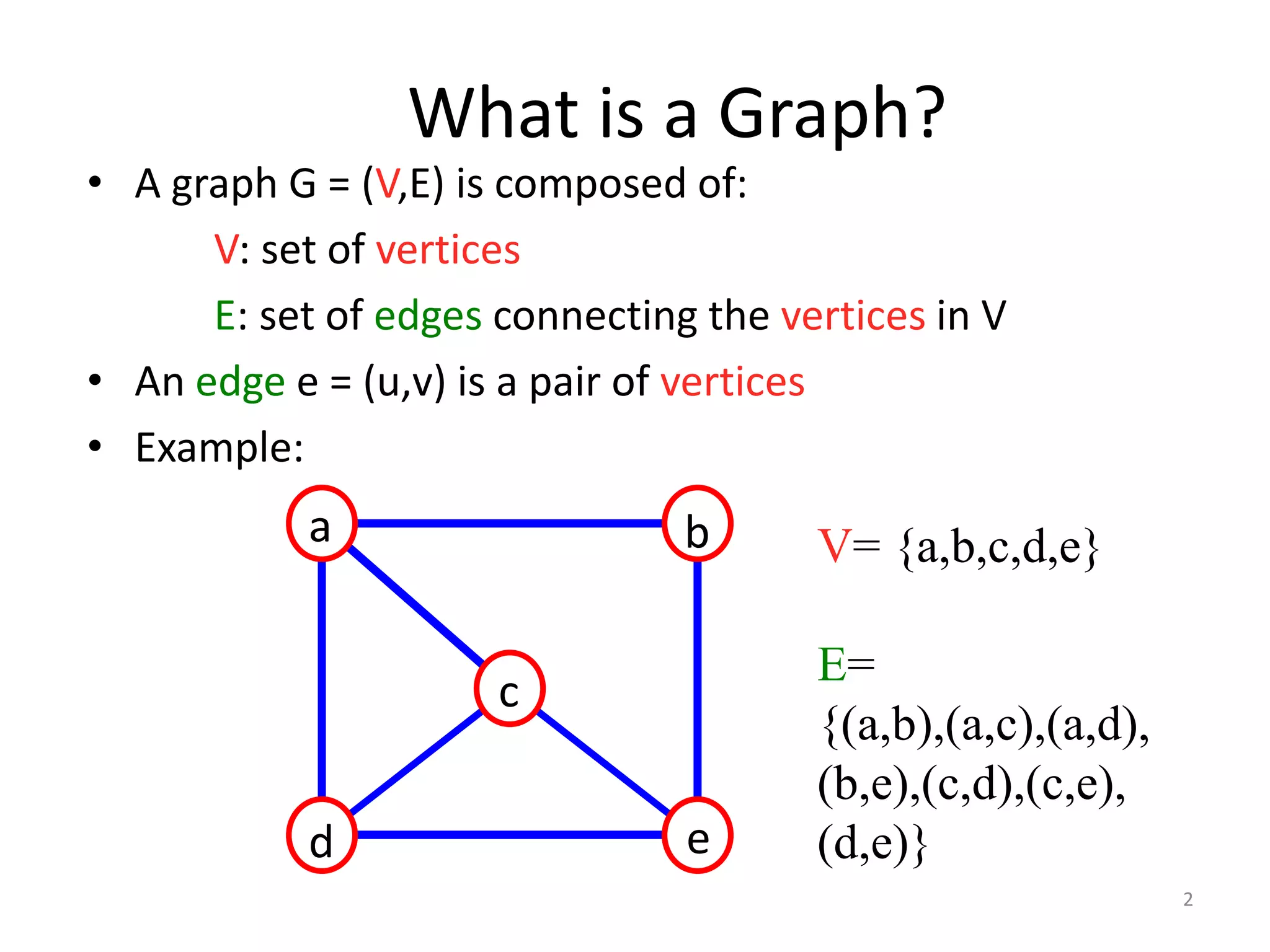
• Let G=(V,E) be a graph with n vertices.
• The adjacency matrix of G is a two-dimensional
n by n array, say adj_mat
• If the edge (vi, vj ) is in E(G), adj_mat[i][j]=1
• If there is no such edge in E(G), adj_mat[i][j]=0
• The adjacency matrix for an undirected graph is
symmetric
• The adjacency matrix for a digraph
need not be symmetric](https://image.slidesharecdn.com/6-201004092731/75/6-Graphs-15-2048.jpg)

![17
Merits of Adjacency Matrix
From the adjacency matrix, to determine the
connection of vertices is easy
The degree of a vertex is
For a digraph (= directed graph), the row sum is
the out_degree, while the column sum is the
in_degree
adj mat i j
j
n
_ [ ][ ]
0
1
ind vi A j i
j
n
( ) [ , ]
0
1
outd vi A i j
j
n
( ) [ , ]
0
1](https://image.slidesharecdn.com/6-201004092731/75/6-Graphs-17-2048.jpg)


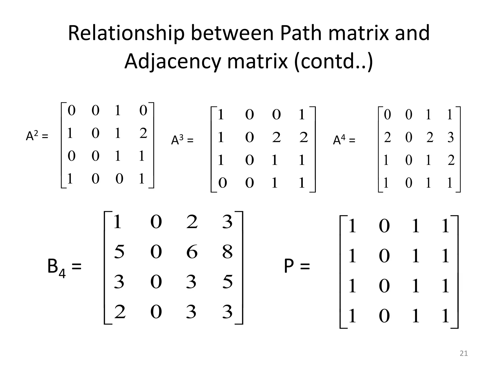


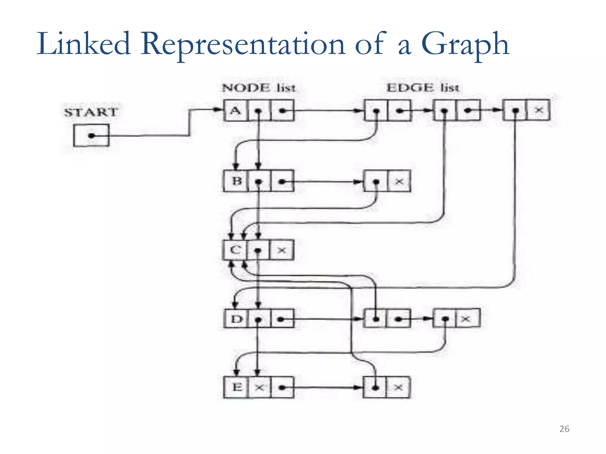


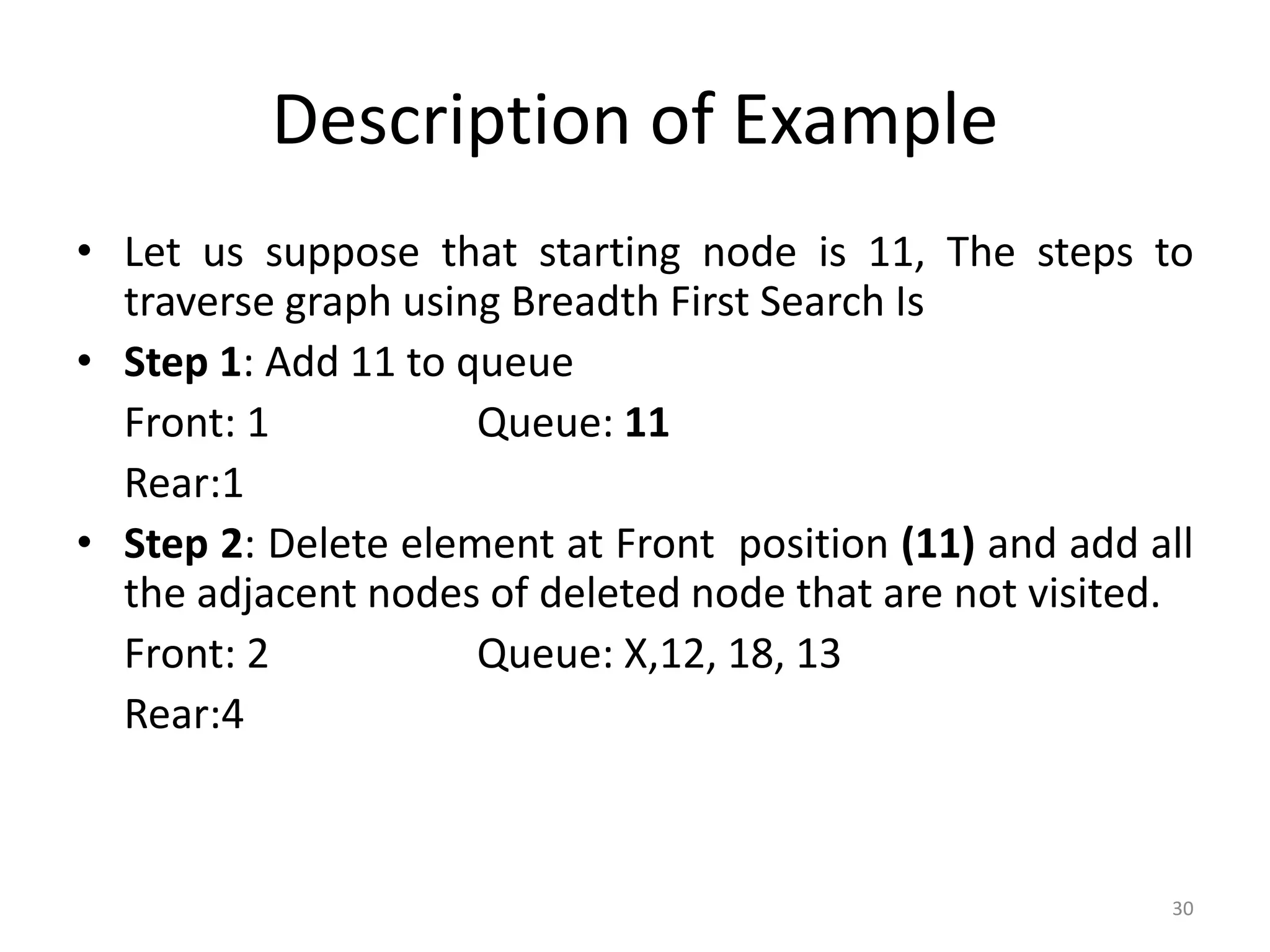
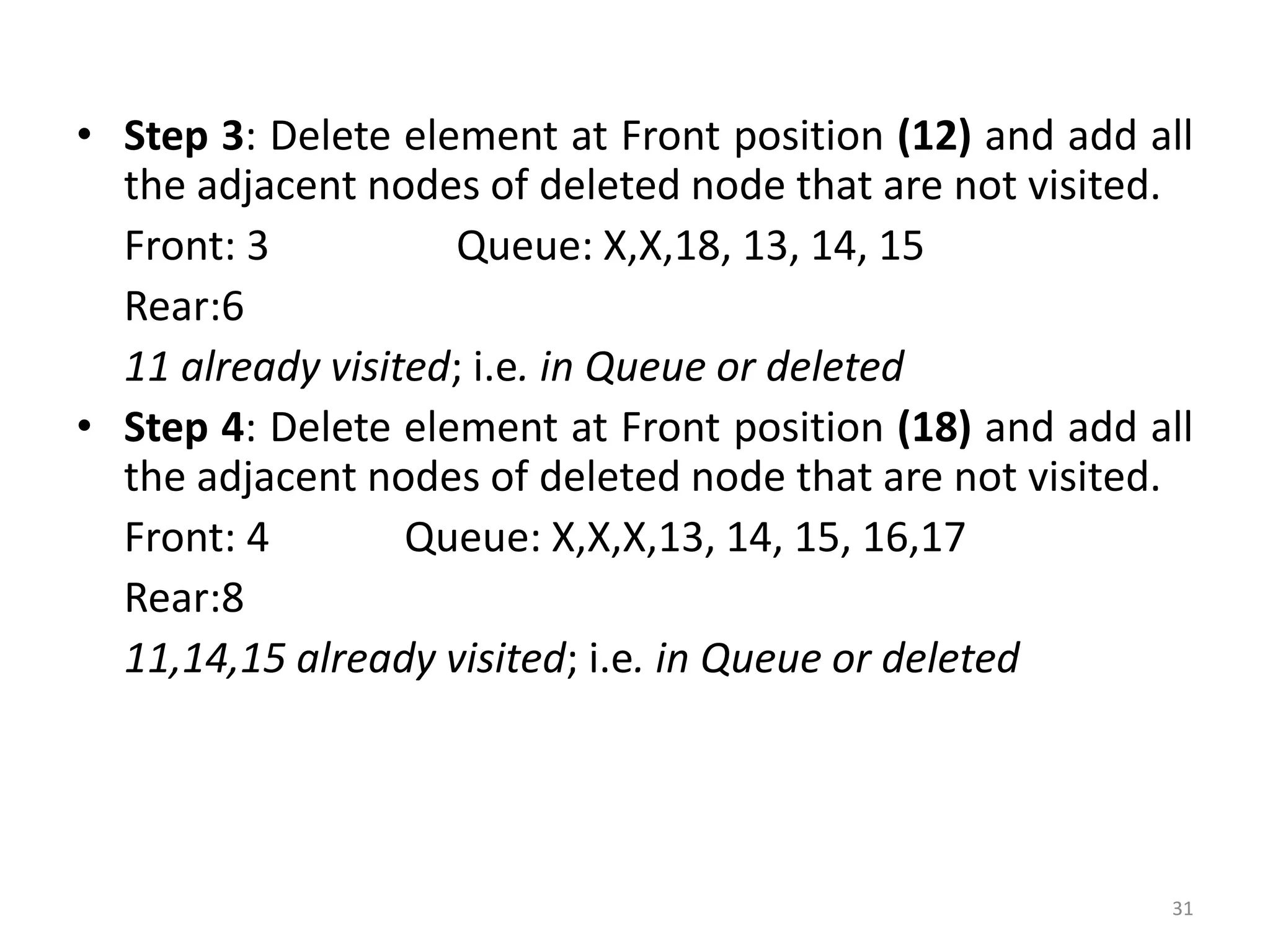


The document defines and explains basic graph terminology and representations. It begins by defining what a graph is composed of, including vertices and edges. It then discusses directed vs undirected graphs and provides examples. It also covers basic graph terminology such as adjacent nodes, degree, paths, cycles, and more. Finally, it discusses different ways of representing graphs, including adjacency matrices, adjacency lists, and traversing graphs using breadth-first and depth-first search algorithms.