Downloaded 124 times
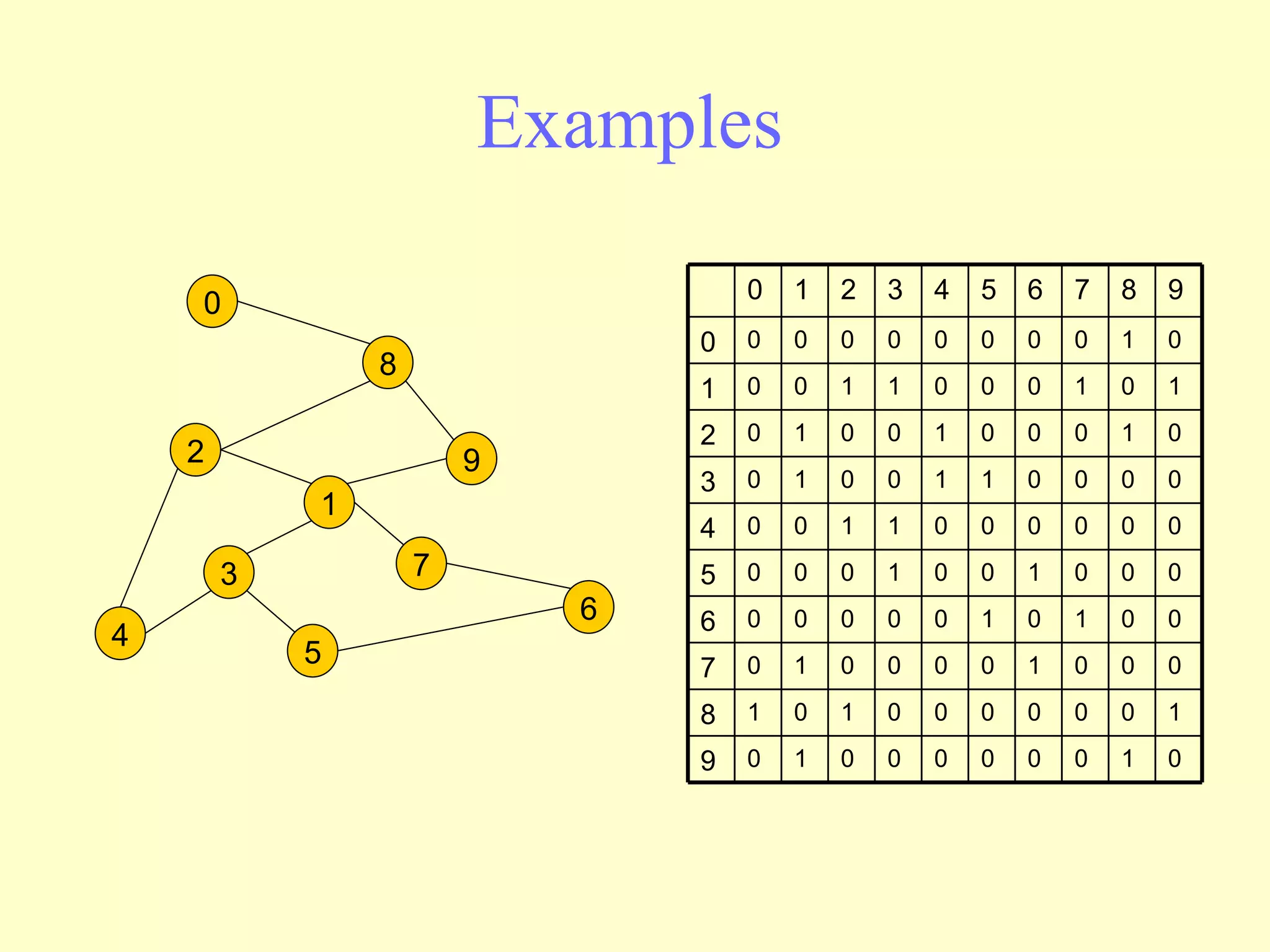
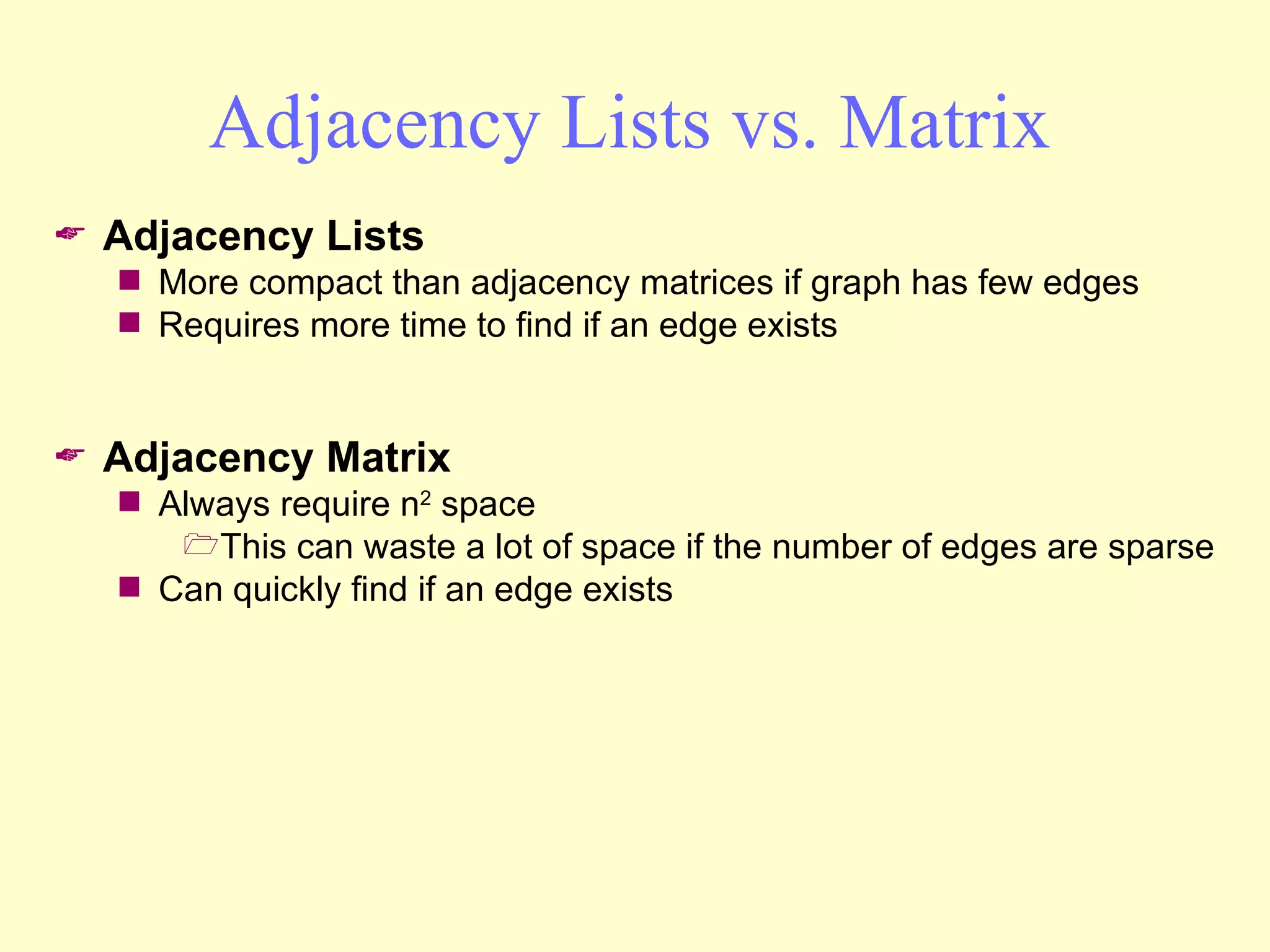
![Adjacency Matrix 2D array A[0..n-1, 0..n-1], where n is the number of vertices in the graph Each row and column is indexed by the vertex id. - e,g a=0, b=1, c=2, d=3, e=4 An array entry A [i] [j] is equal to 1 if there is an edge connecting vertices i and j. Otherwise, A [i] [j] is 0. The storage requirement is Θ (n 2 ). Not efficient if the graph has few edges. We can detect in O(1) time whether two vertices are connected.](https://image.slidesharecdn.com/graphs-110225222859-phpapp02/75/Graphs-7-2048.jpg)
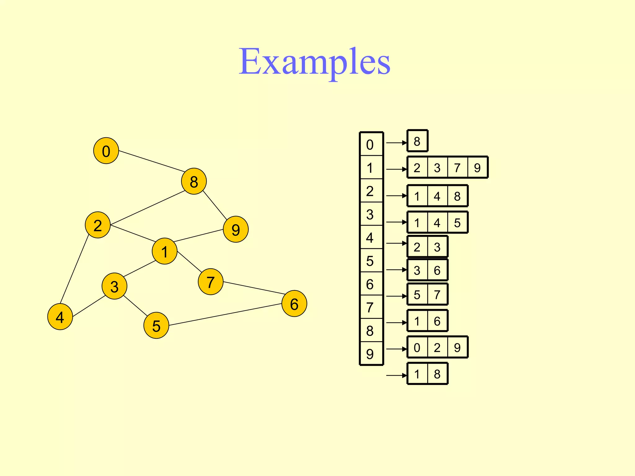
![Adjacency list The adjacency list is an array A[0..n-1] of lists, where n is the number of vertices in the graph. Each array entry is indexed by the vertex id (as with adjacency matrix) The list A[i] stores the ids of the vertices adjacent to i.](https://image.slidesharecdn.com/graphs-110225222859-phpapp02/75/Graphs-8-2048.jpg)
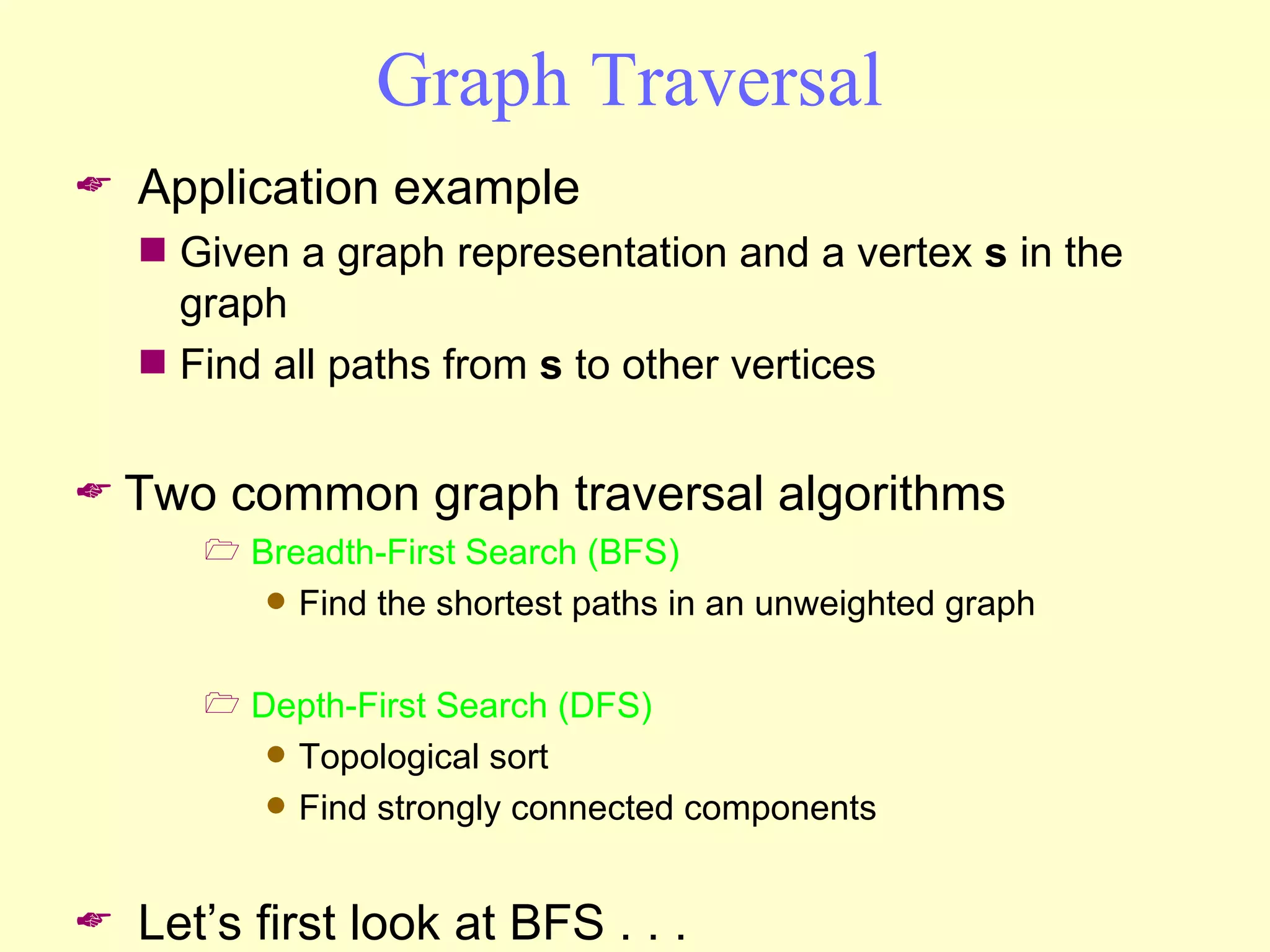
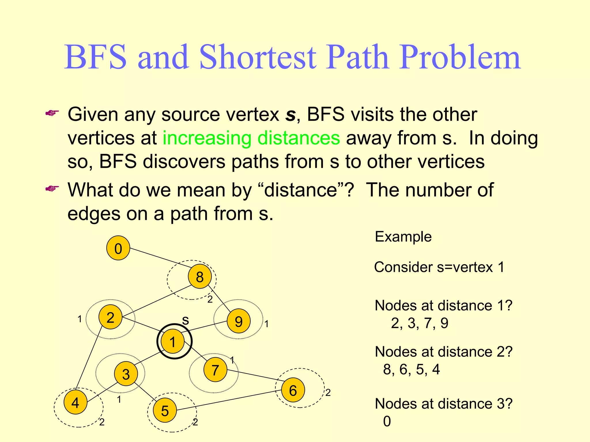
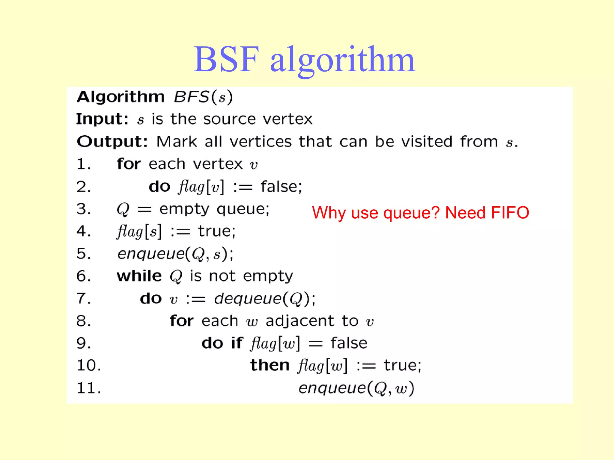
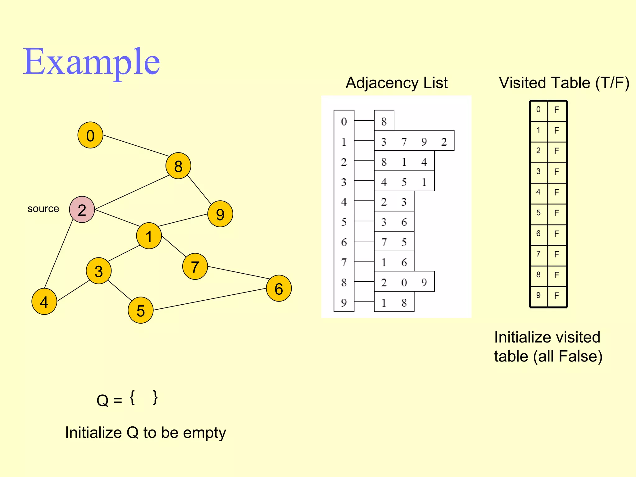
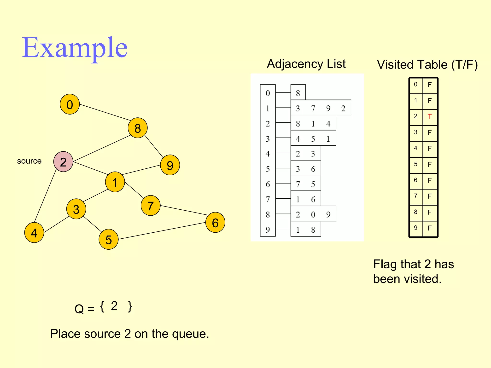
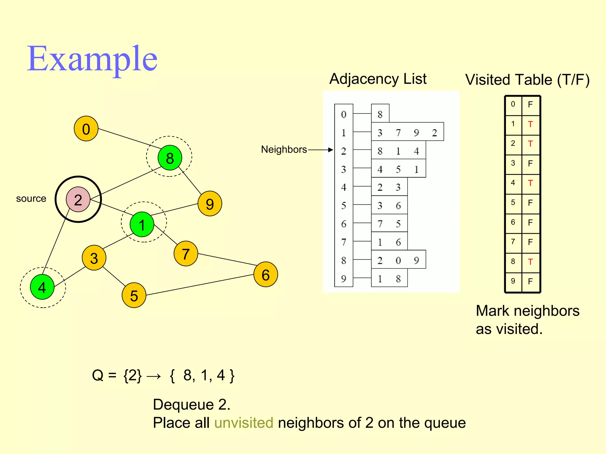
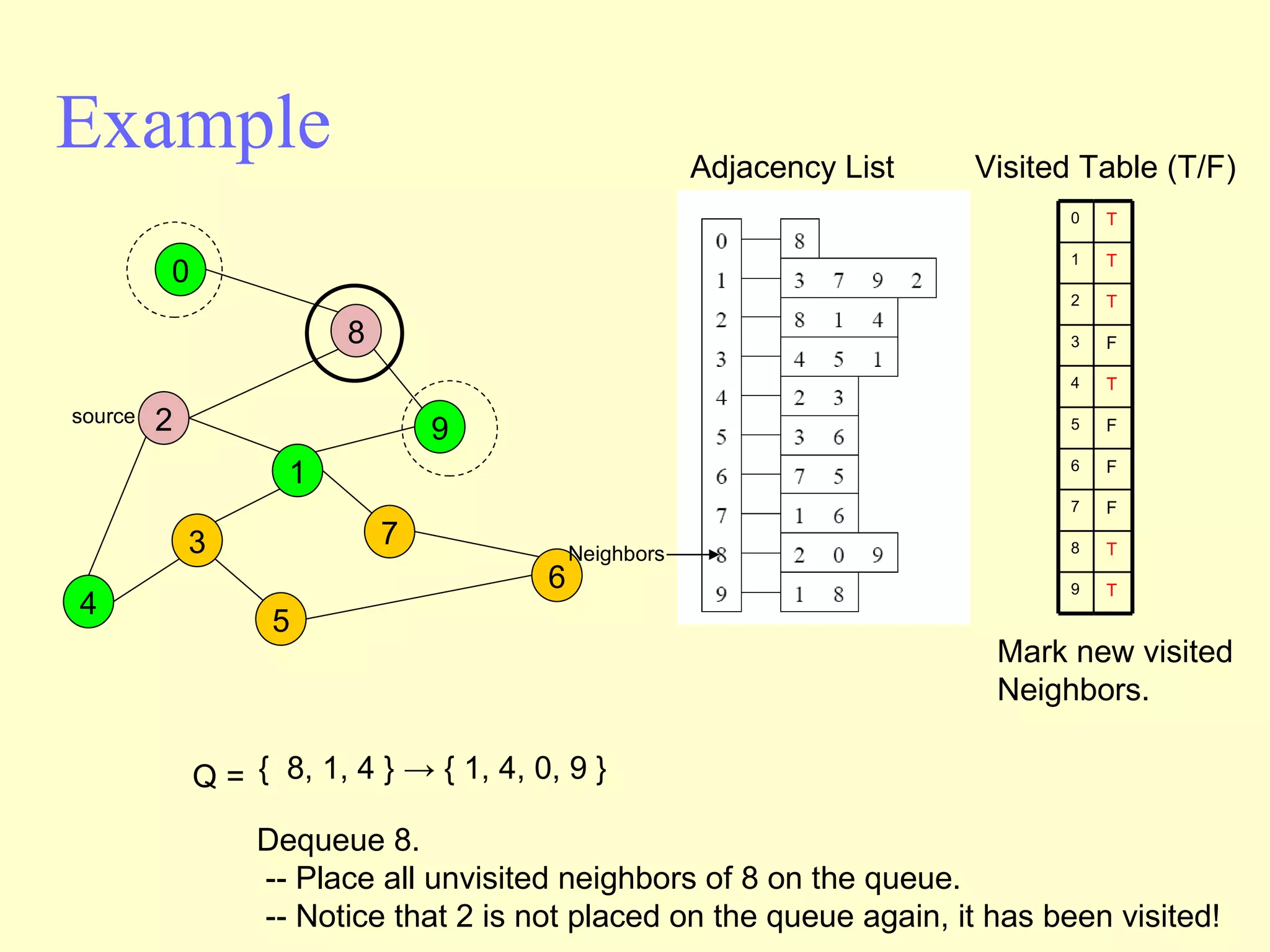
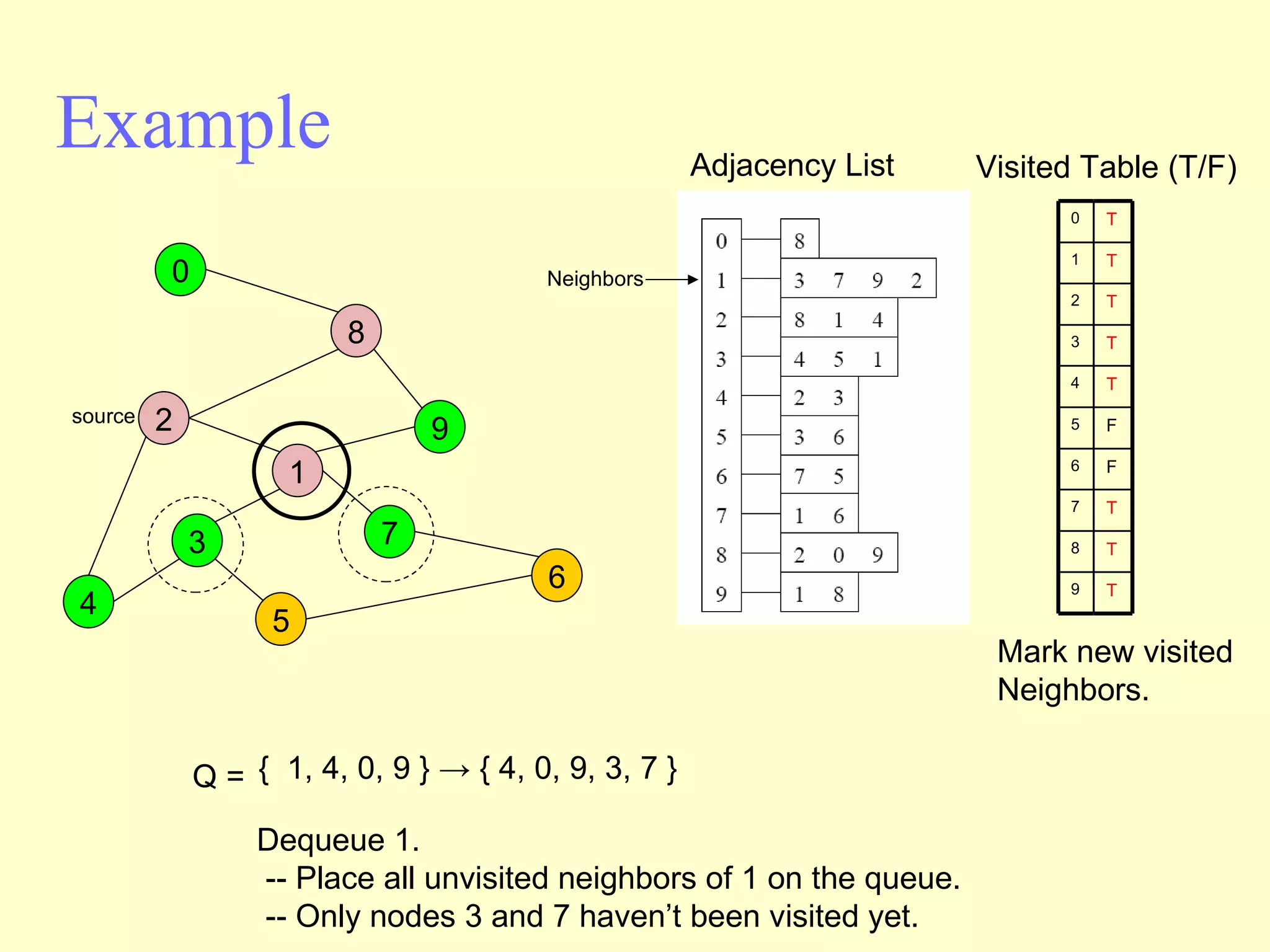
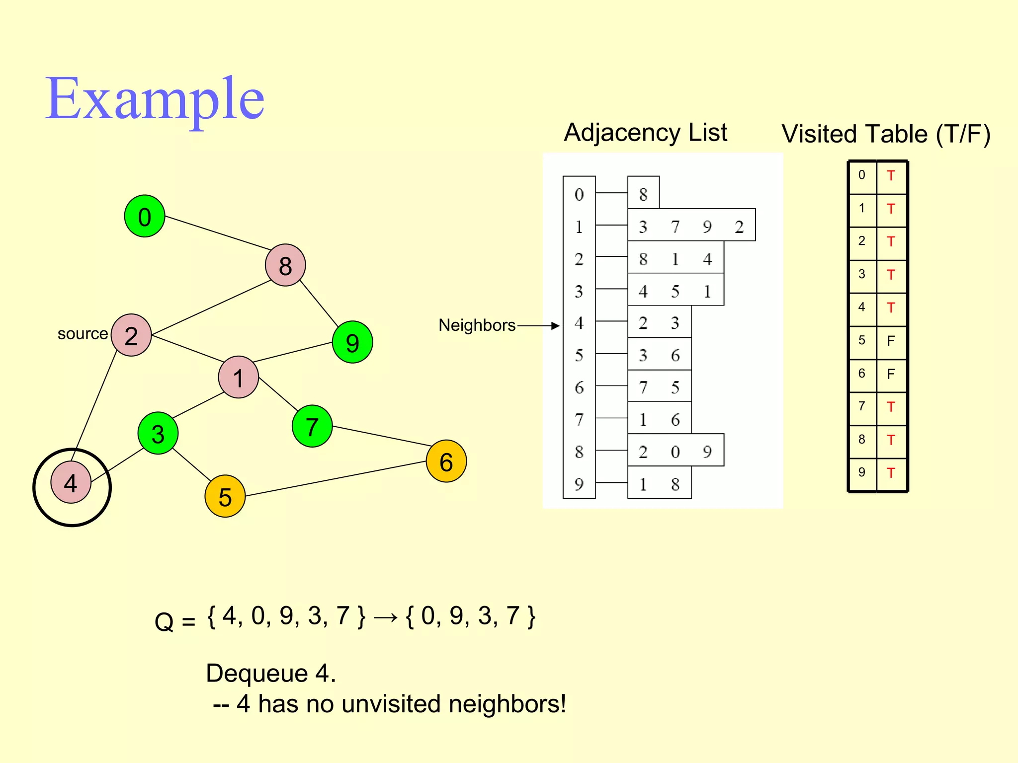
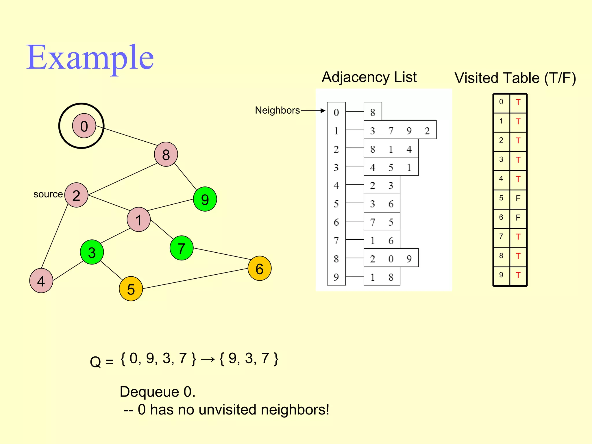
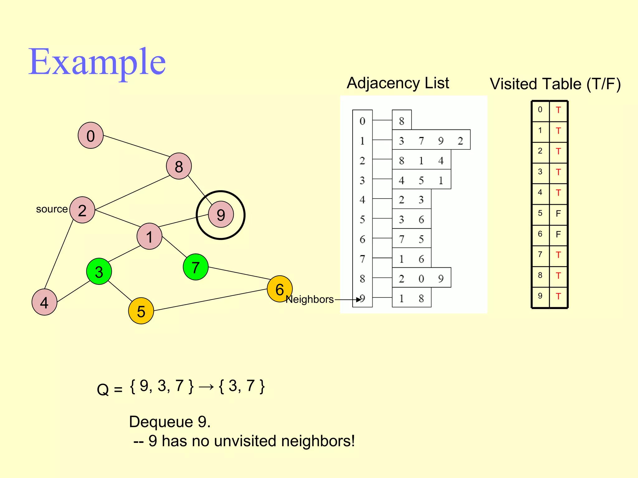
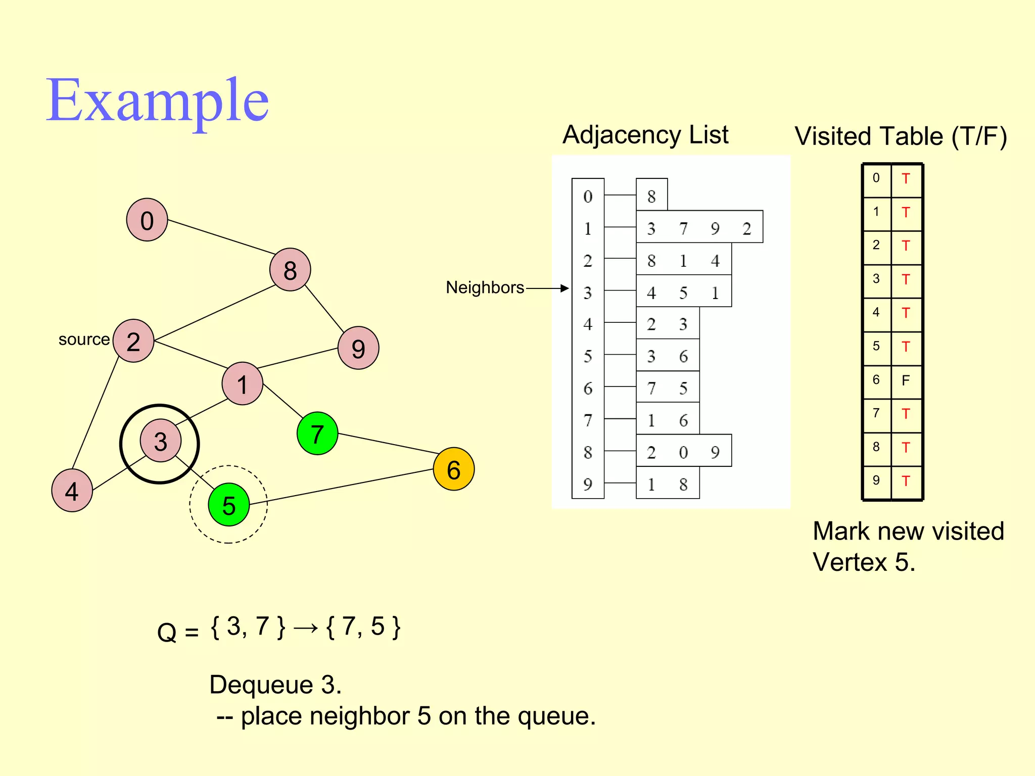
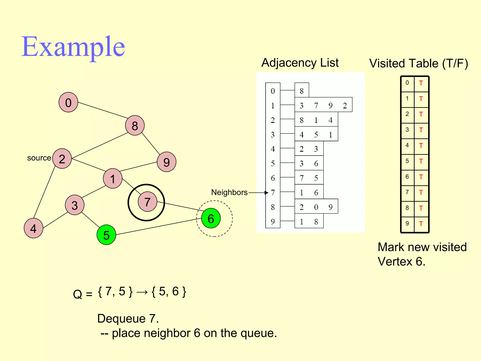
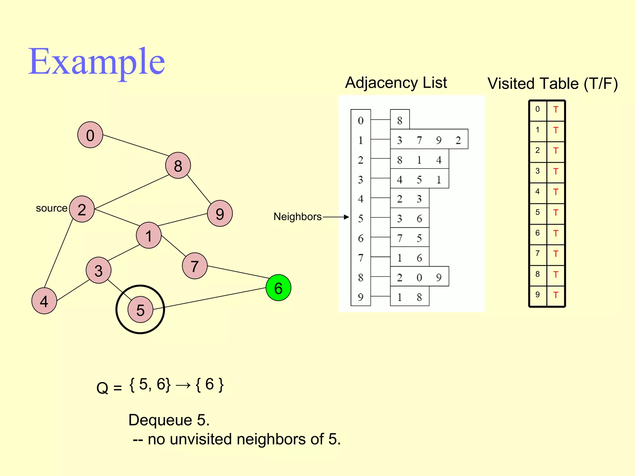
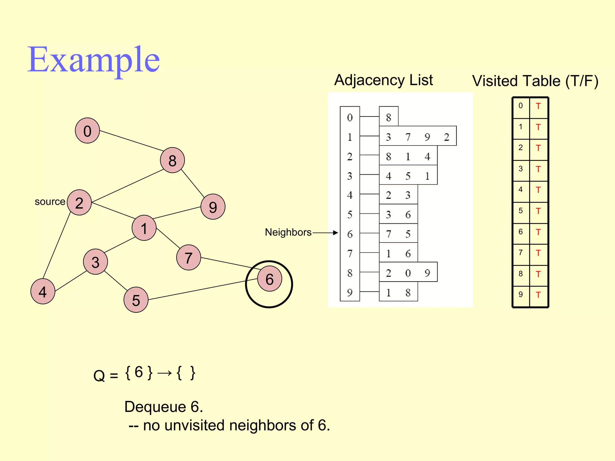
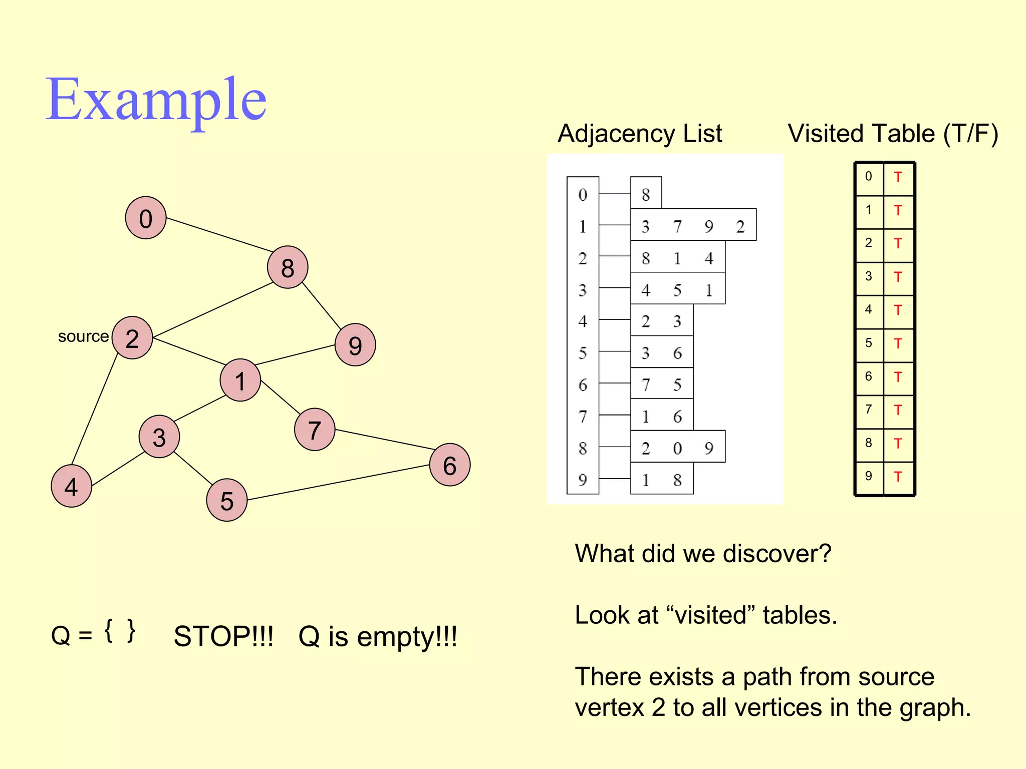
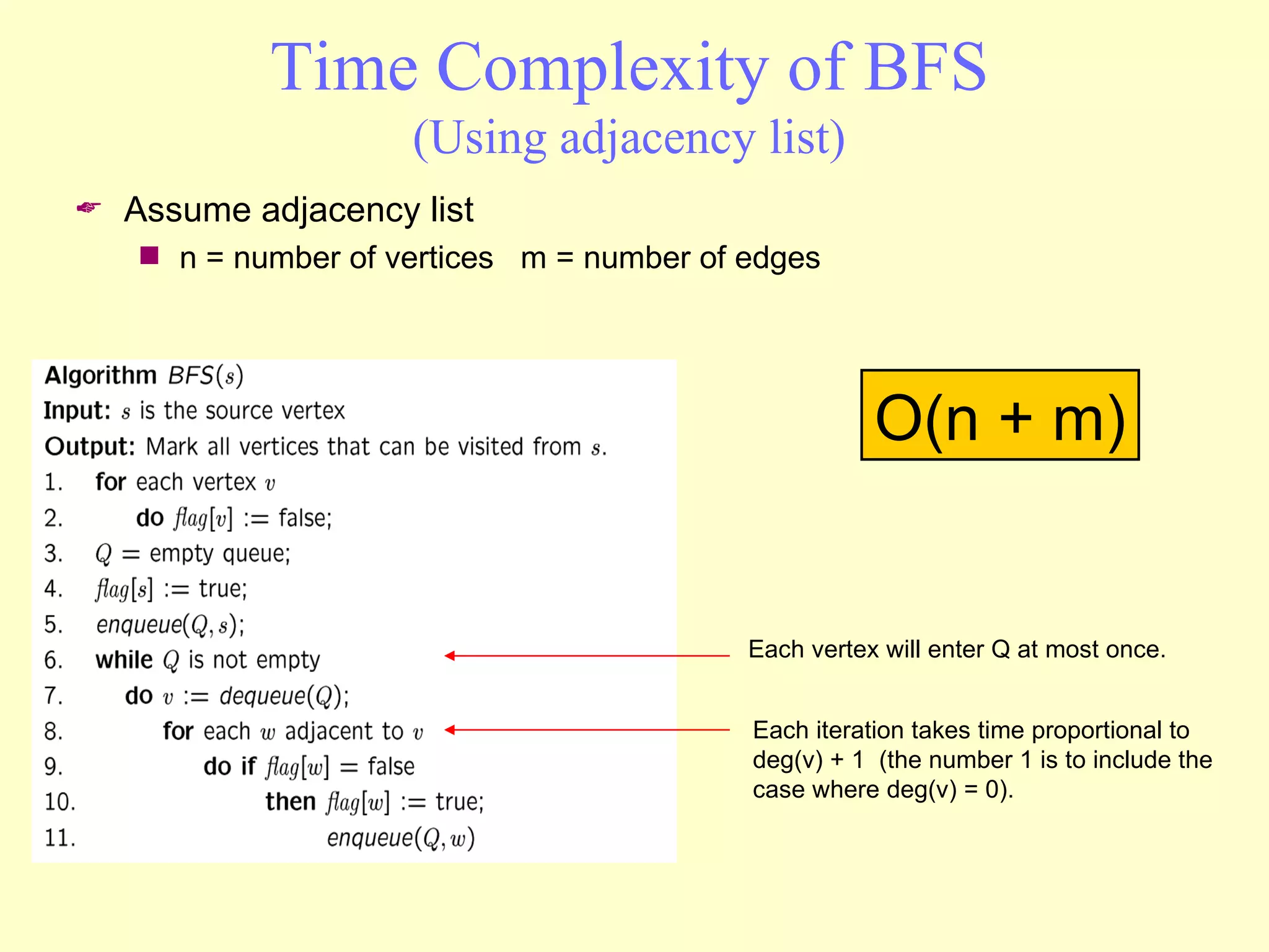
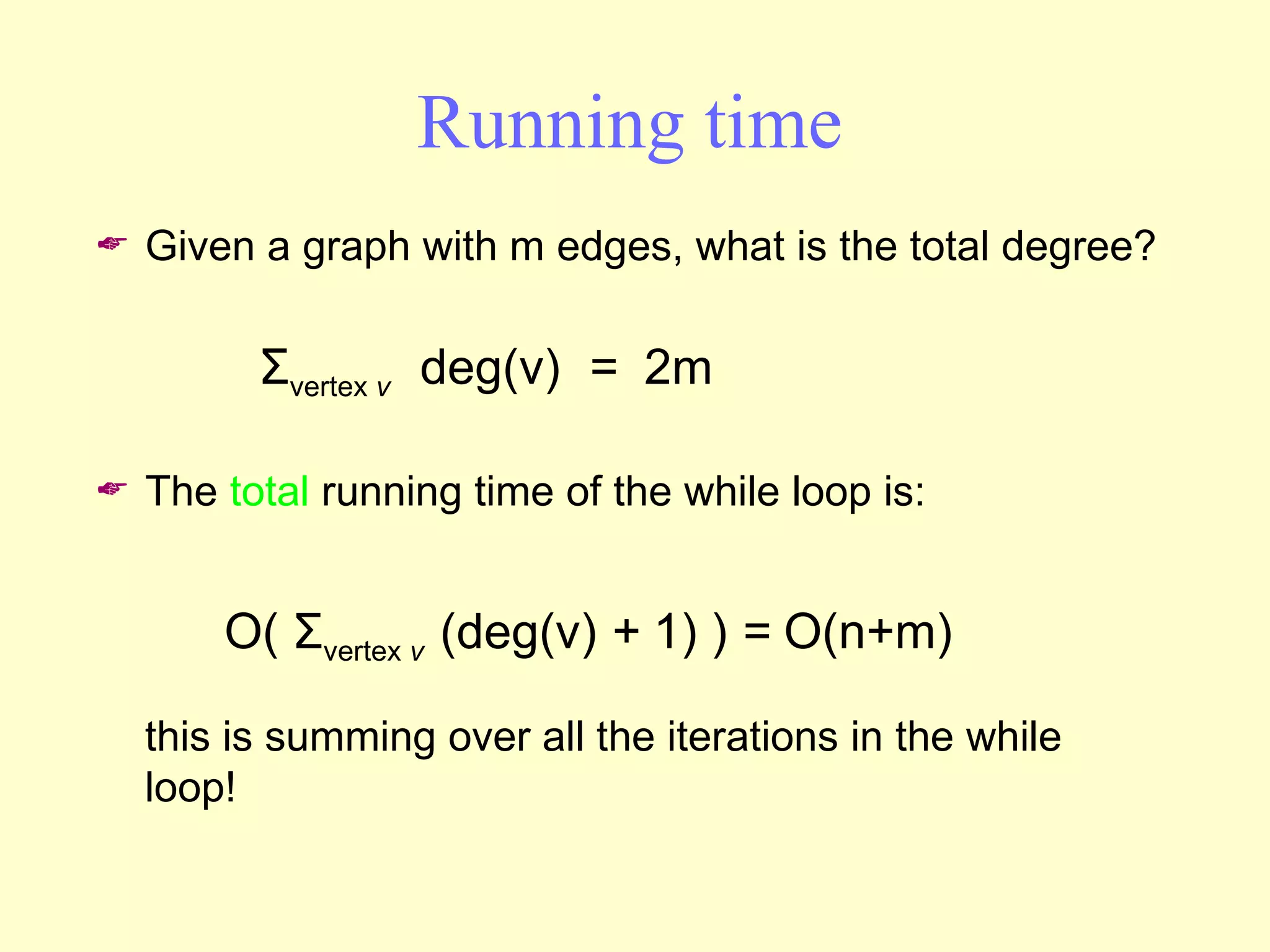

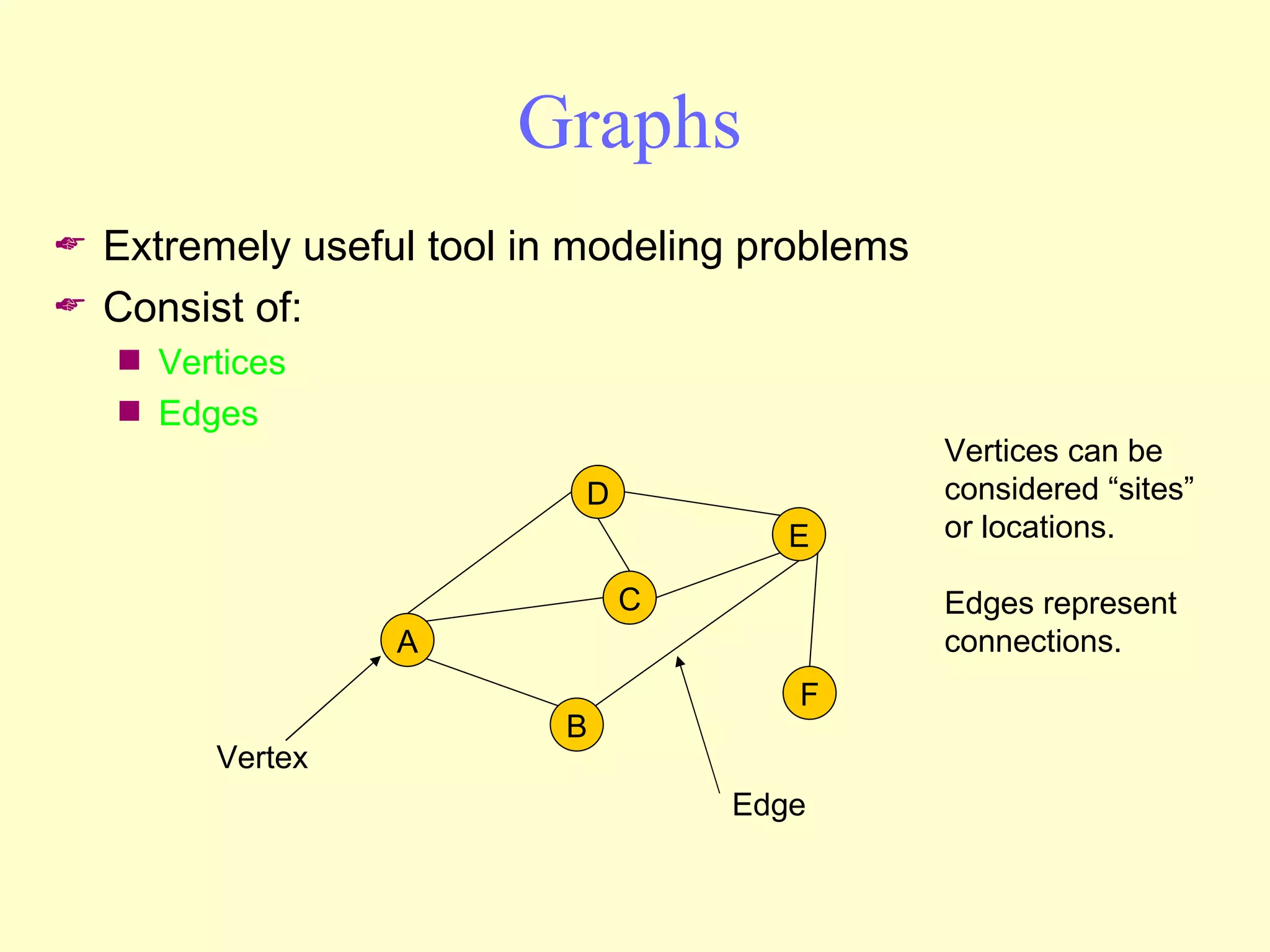
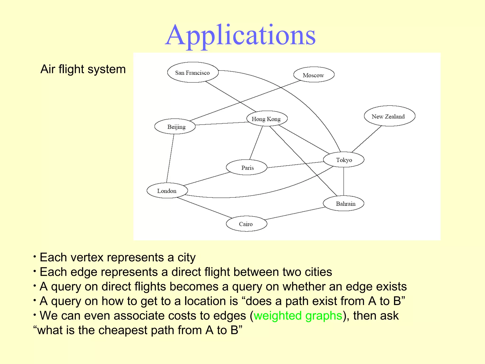
Graphs are useful tools for modeling problems and consist of vertices and edges. Breadth-first search (BFS) is an algorithm that visits the vertices of a graph starting from a source vertex and proceeding to visit neighboring vertices first, before moving to neighbors that are further away. BFS uses a queue to efficiently traverse the graph and discover all possible paths from the source to other vertices, identifying the shortest paths in an unweighted graph. The time complexity of BFS on an adjacency list representation is O(n+m) where n is the number of vertices and m is the number of edges.


![Data Structures - Lecture 10 [Graphs]](https://cdn.slidesharecdn.com/ss_thumbnails/datastructures-lecture10graphs-150305004608-conversion-gate01-thumbnail.jpg?width=640&height=640&fit=bounds)