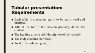
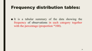
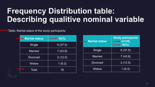
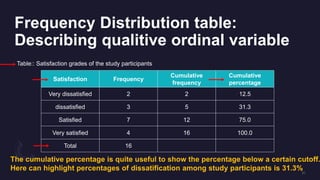
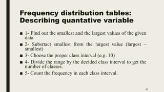
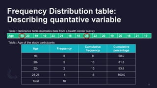
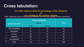
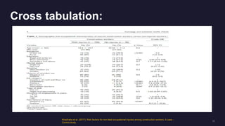
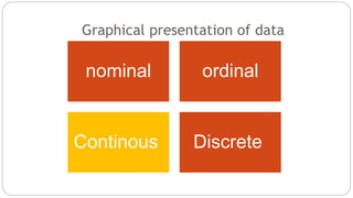
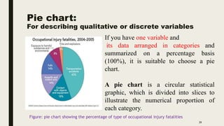
The document discusses data distribution and presentation. It covers topics like the normal distribution curve, calculating probabilities using the standardized normal distribution table, and presenting data through tables and graphs. Specifically, it provides details on creating frequency distribution tables for qualitative and quantitative variables. It also discusses cross tabulation and different types of graphs like pie charts, simple bar charts, and multiple bar charts for presenting categorical data.

1. DATA DISTRIBUTION
AND PRESENTATION
Nada Mohamed Radwan Elhadidy
1

2. Agenda
Data Distribution
Identify the concept of probability
Recognize Normal distribution curve and
its characteristics
Calculate the probabilities as areas
under the curve by using Standardized
Normal Distribution table
Deviation from normality

3. Introduction
• Every variable to be analyzed in a
dataset has both type and distribution.
• Distribution are the building blocks of
statistics, since the correct identification
of a distribution usually allows the
statistician to choose which proper
statistical test should be used to test
statistical significance.

4. Distributions
■ Distributions are statistical constructs that attempt to
describe how probability behaves in certain regions.
Briefly, probability is the likelihood of specific event
happening.
Example: What is the probable percentage of students
scored less than 49? It is 40.0 % of the students
4
Handbook of clinical research :design, statistics, implementation, 2014, flora et al

5. Normal (Gaussian) Distribution
■ It is the most important probability distribution.
■ It is important tool in analysis of epidemiological data
& management science.
■ It is called “Gaussian” The noted statistician professor
Gauss developed this.
What does a Gaussian distribution tell us?
5

6. Normal (Gaussian) Distribution
6

7. Normal (Gaussian) Distribution
7

8. Normal (Gaussian) Distribution
8
Characteristic of the normal
distribution curve:
1. It is bell shaped.
2. The curve rises to its peak at
the mean where mean
=median = mode.
3. Symmetrically distributed on
both sides of mean

9. Normal (Gaussian) Distribution
9
Characteristic of the normal
distribution curve:
4. The area starts from -ve to
+ve and the two edges of the
curve do not meet X line except
at infinity
5.The X axis is divided
according to standard deviation
(SD) into about 3 SD.

10. Normal (Gaussian) Distribution
10
Characteristic of the normal
distribution curve:
6. The values lying within the
interval
(µ ± 1σ) (χ̅± SD) = 68% of all
values
(µ ± 2σ) (χ̅± 2SD) = 95% of all
values.
(µ ± 3σ) (χ̅± 3SD) = all values
(99.7%).

11. Normal (Gaussian) Distribution
11
Characteristic of the normal
distribution curve:
7. The area under normal curve
above the X-axis = 100.0%,
each half = 50.0%.

12. Normal (Gaussian) Distribution
E.g. According to Gaussian distribution, Determine the intervals and calculate
the number of observations in each interval for the normally distributed
dataset, n= 90, χ̅= 50, SD= 5?
Intervals
(χ̅± 1 SD) = 50 ± 5 (45 to 55) includes 68.2% of all values equal (61 observations)
(χ̅± 2 SD) = 50 ± 2(5) (40 to 60) includes 95.4% of all values equal (86 observations)
(χ̅± 3 SD) = 50 ± 3(5) (35 to 65) includes 99.7% of the values equal (90 observations)
12

13. Standardized Normal Distribution:
Calculating Probabilities
13

14. Standardized Normal Distribution:
Calculating Probabilities
14

15. Standardized Normal Distribution:
Calculating Probabilities
15
The test birth weights of 3226 babies in hospital has a mean of 3.4 and with a
standard deviation of 0.55. What is the probable percentage of babies scored
less than 2.5?
■ Solution: The z score for the given data is,
z= (2.5 – 3.4)/0.55= - 1.64

16. Standardized Normal Distribution:
Calculating Probabilities
16

17. Standardized Normal Distribution:
Calculating Probabilities
17
The test birth weights of 3226 babies in hospital has a mean of 3.4 and with a
standard deviation of 0.55. What is the probable percentage of babies scored
less than 2.5?
■ Solution: The z score for the given data is,
z= (2.5 – 3.4)/0.55= - 1.64
From the z score table, the fraction of the data within this score is 0.050.
This means 5.0 % of the babies are within the birthweight less than 2.5.

18. Deviation from normality:
Skewed Distribution
18

19. Deviation from normality:
Skewed Distribution
19

20. Deviation from normality:
Skewed Distribution
20

21. Reasons for non normal data
1. Outliers can cause your data the become skewed. The
mean is especially sensitive to outliers.
Advise :Try removing any extreme high or low values
and testing your data again.
2. Overlap of Two or More Processes
Multiple distributions may be combined in your data,
giving the appearance of a bimodal or multimodal
distribution.
Hidden
causes
Frank
causes

22. Reasons for non normal data
3.Insufficient Data
 For example, classroom test results are usually normally distributed.,
if you choose three random students and plot the results on a graph,
you won’t get a normal distribution.
 You might get a uniform distribution (i.e. 62/ 62/ 63) or a skewed
distribution (80 /92/ 99).
 Advise : Increase your sample size.
4.Data may be inappropriately graphed.
 E.g: graphing people’s weights on a scale of 0 to 1000 lbs,
you would have a skewed to the left
5. Values close to zero or natural limit
6. Data Follows a Different Distribution by nature
as follow

23. Normality test
This can be done by many statistical methods
including Kolmogorov-Smirnov test (for large data
sets) and
Shapiro-Wilk test (for small data sets <50) where
data will be considered normally distributed if the
test result is non significant (p value > 0.050) and
data will be considered non-normally distributed
(skewed) if the test result is significant (p value ≤
0.050)
23

24. Normality test
24

25. The mean age±2 standard deviation of a sample of
100 sample equals 55± 10.
Considering that age is normally distributed you are
expected that nearly 95 patients will have their age:
A.Between 45 and 65 years.
B.Between 25 and 85 years.
C.Between 35 and 75 years.
D.Between 55 and 65 years.

26. Serum cholesterol levels in a group of young adults
found to be approximately normally distributed with
mean level 170 mg/dl and standard deviation 8
mg/dl. which of the following intervals include
approximately 68% of serum cholesterol in this
group?
A)160-180 mg/dl
B)162-178 mg/dl
C)150-190 mg/dl
D)154-186 mg/dl
E)140-200 mg/dl

27. Agenda
Tabular presentation
Requirements for tabulation
Frequency distribution tables
Cross tabulations

28. Tabular presentation:
Requirements
■ Each table is a separate entity to be easily read and
interpret.
■ Title at the top of the table to precisely define the
content.
■ The heading gives a brief description of the variable.
■ The body contains the values.
■ Total (row, column, grand).
28

29. Frequency distribution tables:
■ It is a tabular summary of the data showing the
frequency of observations in each category together
with the percentage (proportion *100).
29

30. Frequency Distribution table:
Describing qualitive nominal variable
Marital status N(%)
Single 6 (37.5)
Married 7 (43.8)
Divorced 2 (12.5)
Widow 1 (6.3)
Total 16
Table: Marital status of the study participants
Marital status
Study paricipants
(n=16)
N(%)
Single 6 (37.5)
Married 7 (43.8)
Divorced 2 (12.5)
Widow 1 (6.3)

31. Frequency Distribution table:
Describing qualitive ordinal variable
Satisfaction Frequency
Cumulative
frequency
Cumulative
percentage
Very dissatisfied 2 2 12.5
dissatisfied 3 5 31.3
Satisfied 7 12 75.0
Very satisfied 4 16 100.0
Total 16
Table:: Satisfaction grades of the study participants
The cumulative percentage is quite useful to show the percentage below a certain cutoff.
Here can highlight percentages of dissatification among study participants is 31.3%

32. Frequency distribution tables:
Describing quantative variable
■ 1- Find out the smallest and the largest values of the given
data
■ 2- Subsrtact smallest from the largest value (largest –
smallest)
■ 3- Choose the proper class interval (e.g. 10)
■ 4- Divide the range by the decided class interval to get the
number of classes.
■ 5- Count the frequency in each class interval.
32

33. Frequency Distribution table:
Describing quantative variable
Table:: Reference table illustrates data from a health center survey
Age 18 20 19 19 23 21 18 18 26 22 20 19 20 18 21 19
Table:: Age of the study participants
Age Frequency
Cumulative
frequency
Cumulative
percentage
18- 8 8 50.0
20- 5 13 81.3
22- 2 15 93.8
24-26 1 16 100.0
Total 16

34. Cross tabulation:
Satisfaction level
Study participants
Total
Gender
Male Female
Very dissatisfied 41 22 63
dissatisfied 24 18 42
Unsure 22 31 53
Satisfied 40 24 64
Very satisfied 15 12 27
Total 142 107 249
Table: Satisfaction level of the provided healthcare services within gender of study participants
It is often useful to show the percentage of the categories
of
one variable by the another variable.

35. Cross tabulation:
Khashaba et al. (2017): Risk factors for non-fatal occupational injuries among construction workers: A case –
Control study.

36. Graphical presentation:
36

37. Graphical presentation of data
nominal ordinal
Continous Discrete

38. Agenda

39. Pie chart:
For describing qualitative or discrete variables
39
If you have one variable and
its data arranged in categories and
summarized on a percentage basis
(100%), it is suitable to choose a pie
chart.
A pie chart is a circular statistical
graphic, which is divided into slices to
illustrate the numerical proportion of
each category.
Figure: pie chart showing the percentage of type of occupational injury fatalities

40. Simple bar chart:
For describing qualitative or discrete variables
40
If you have one variable and
its data arranged in categories and
summarized on a percentage basis, it is
suitable to choose a simple bar chart.
Figure: simple bar chart showing the frequency distribution of type of burns in hospital

41. Simple bar chart:
For describing qualitative or discrete variables
41
This is a chart with frequency on the vertical
axis and category on the horizontal axis.
A bar is drawn for each category, its length
being proportional to the frequency in that
category.
The bars are separated by small gaps to indicate
that the data are categorical or discrete
Figure: simple bar chart showing the frequency distribution of type of burns in hospital

42. Multiple (clustered) bar chart:
For describing qualitative or discrete variables
42
If you divide the sample into different (two
or more) groups, and
you want to compare category proportion
within each group (e.g. frequency of girls
vs frequency of boys in group A) and
you can use the multiple bar chart.
Figure: multiple bar chart showing the frequency distribution of girls and boys within groups

43. Multiple (clustered) bar chart:
For describing qualitative or discrete variables
43
If you divide the sample into different (two
or more) groups, and
you want to comparealso the relative sizes
of the groups within each category
(e.g. frequency of girls in group A vs
Group B vs Group C vs group
D),
you can use the multiple bar chart.
Figure: multiple bar chart showing the frequency distribution of girls and boys within groups

44. Component (stacked) bar chart:
For describing qualitative or discrete variables
44
If you divide the sample into different (two
or more) groups, and
you want to compare the relative sizes of
the groups within each category(e.g.
frequency of blood group A in city X vs
city Y vs city Z),
you can use the component bar chart

45. Component (stacked) bar chart:
For describing qualitative or discrete variables
45
If you divide the sample into different (two
or more) groups, and
you want to compare category proportion
within each group (e.g. frequency of blood
group A vs B vs AB vs O in city X),
you can use the component bar chart
Figure: component bar chart showing the frequency distribution of blood groups across some Egyptian citie

46. Histogram:
For describing continuous variables
46
A histogram is a graph of the
frequency distribution of a continuous
variable.
A histogram looks like a bar chart but
without any gaps between adjacent bars
to emphasize the continuous nature of
the variable and to represent the number
of observations for each class interval
in the distribution.
Figure: Histogram showing the frequency distribution of weights of patients

47. Frequency polygon:
For describing continuous variables
47
Mid points of upper bases of rectangles
are connected by a series of straight
lines.
Figure: frequency polygon showing the frequency distribution of heights of patients

48. Smooth curve:
For describing continuous variables
48
Figure: Histogram with normal distribution curve
taking bell-shaped curve
Figure: histogram with skewed curve

49. Box and whisker plot:
For describing continuous variables
49
Figure: box and whisker plot showing median (interquartile range) of birth weights across different types of d

50. Scatter diagram:
For describing continuous variables
50
It is useful for analyzing
the relations between
two variables.
One variable is plotted
on the horizontal axis
and the other is plotted
on the vertical axis.

51. Graphical presentation:
The most common types of graphical presentation:
■ For describing qualitative or discrete variables
are bar and pie charts.
■ For describing continuous variables are
histogram, frequency polygon, smooth curves,
box and whisker plot.
■ For relation between variables are scatter
diagram
51

52. Which of the following data is best described by
Histogram?
a. Height of infants in cm of
b. Gender of a group of patients
c. Type of treatment
d. Severity of pain
e. Height of patients (short-average-tall)
Questions

53. Graph showing the relation between serum
calcium and bone mineral density variables is
called:
(a) Scatter diagram
(b) Frequency polygon
(c) Picture chart
(d) Histogram
(e) pie chart
Questions

54. You are preparing a report to present
mortality & morbidity from covid 19
according to age groups(<20 years,20-
40,>40) during the last 12 months. Which
graph best describes these data?
A)Simple bar chart
B)Multiple bar chart
C)Frequency polygon
D)Histogram
E)Pie chart
Questions

55. 55