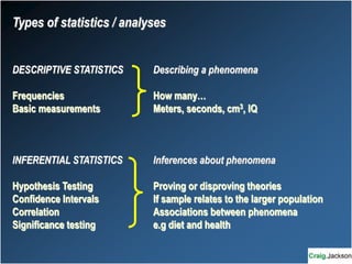
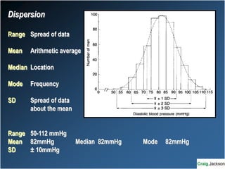
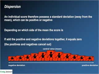
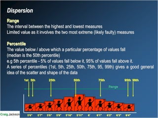
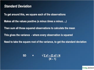
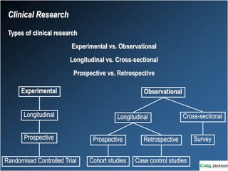
The following lecture has been approved for
University Undergraduate Students
This lecture may contain information, ideas, concepts and discursive anecdotes
that may be thought provoking and challenging
It is not intended for the content or delivery to cause offence
Any issues raised in the lecture may require the viewer to engage in further
thought, insight, reflection or critical evaluation
Background to Statistics
for
non-statisticians
Craig Jackson
Prof. Occupational Health Psychology
Faculty of Education, Law & Social Sciences
BCU
craig.jackson@bcu.ac.uk
Keep it simple
“Some people hate the very name of statistics but.....their power of
dealing with complicated phenomena is extraordinary. They are the
only tools by which an opening can be cut through the formidable
thicket of difficulties that bars the path of those who pursue the science
of man.”
Sir Francis Galton, 1889
How Many Make a Sample?
“8 out of 10 owners who expressed a preference, said their cats
preferred it.”
How confident can we be about such statistics?
8 out of 10?
80 out of 100?
800 out of 1000?
80,000 out of 100,000?
Types of Data / Variables
Continuous Discrete
BP Children
Height Age last birthday
Weight colds in last year
Age
Ordinal Nominal
Grade of condition Sex
Positions 1st 2nd 3rd Hair colour
“Better- Same-Worse” Blood group
Height groups Eye colour
Age groups
Conversion & Re-classification
Easier to summarise Ordinal / Nominal data
Cut-off Points (who decides this?)
Allows Continuous variables to be changed into Nominal variables
BP > 90mmHg = Hypertensive
BP =< 90mmHg = Normotensive
Easier clinical decisions
Categorisation reduces quality of data
Statistical tests may be more “sensational”
Good for summaries Bad for “accuracy”
BMI
Obese vs Underweight
Types of statistics / analyses
DESCRIPTIVE STATISTICS Describing a phenomena
Frequencies How many…
Basic measurements Meters, seconds, cm3, IQ
INFERENTIAL STATISTICS Inferences about phenomena
Hypothesis Testing Proving or disproving theories
Confidence Intervals If sample relates to the larger population
Correlation Associations between phenomena
Significance testing e.g diet and health
Multiple Measurement
or….
why statisticians and love don’t mix
25 cells
22 cells
24 cells
21 cells
Total = 92 cells
Mean = 23 cells
SD = 1.8 cells
26
25
24
23
22
21
20
N Age IQ
1 20 100
2 20 100
3 20 100
4 20 100
5 20 100
6 20 100
7 20 100
8 20 100
9 20 100
10 20 100
Total 200 1000
Mean 20 100
SD 0 0
N Age IQ
1 18 100
2 20 110
3 22 119
4 24 101
5 26 105
6 21 113
7 19 120
8 25 119
9 20 114
10 21 101
Total 216 1102
Mean 21.6 110.2
SD ± 4.2 ± 19.2
N Age IQ
1 18 100
2 20 110
3 22 119
4 24 101
5 26 105
6 21 113
7 19 120
8 25 119
9 20 114
10 45 156
Total 240 1157
Mean 24 115.7
SD ± 8.5 ± 30.2
Small samples spoil research
Central Tendency
Mode
Median Mean
Patient comfort rating
10 9 8 7 6 5 4 3 2 1
31 27 70 121 140 129 128 90 80 62
Frequency
Dispersion
Range Spread of data
Mean Arithmetic average
Median Location
Mode Frequency
SD Spread of data
about the mean
Range 50-112 mmHg
Mean 82mmHg Median 82mmHg Mode 82mmHg
SD ± 10mmHg
Dispersion
An individual score therefore possess a standard deviation (away from the
mean), which can be positive or negative
Depending on which side of the mean the score is
If add the positive and negative deviations together, it equals zero
(the positives and negatives cancel out)
central value (mean)
negative deviation positive deviation
5’6” 5’7” 5’8” 5’9” 5’10” 5’11” 6’ 6’1” 6’2” 6’3” 6’4”
Range
1st 5th 25th 50th 75th 95th 99th
Dispersion
Range
The interval between the highest and lowest measures
Limited value as it involves the two most extreme (likely faulty) measures
Percentile
The value below / above which a particular percentage of values fall
(median is the 50th percentile)
e.g 5th percentile - 5% of values fall below it, 95% of values fall above it.
A series of percentiles (1st, 5th, 25th, 50th, 75th, 95, 99th) gives a good general
idea of the scatter and shape of the data
Standard Deviation
To get around this, we square each of the observations
Makes all the values positive (a minus times a minus….)
Then sum all those squared observations to calculate the mean
This gives the variance - where every observation is squared
Need to take the square root of the variance, to get the standard deviation
SD =  Σ x2 – (Σ x)2 / N
(N – 1)
Non Normal Distribution
Some distributions fail to be symmetrical
If the tail on the left is longer than the right,
the distribution is negatively skewed (to the left)
If the tail on the right is longer than the left, the
distribution is positively skewed
(to the right)
Grouped Data
Normal Distribution
SD is useful because of the shape of many distributions of data.
Symmetrical, bell-shaped / normal / Gaussian distribution
central value (mean)
3 SD 2 SD 1 SD 0 SD 1 SD 2 SD 3 SD
Normal Distributions
Standard Normal Distribution has a mean of 0 and a standard deviation of 1
The total area under the curve amounts to 100% / unity of the observations
Proportions of observations within any given range can be obtained from the
distribution by using statistical tables of the standard normal distribution
95% of measurements / observations lie within 1.96 SD’s either side of the
mean
balls dropped through a
succession of metal pins…..
…..a normal distribution
of balls
do not have a normal
distribution here. Why?
Quincunx machine 1877
The distribution derived from the
quincunx is not perfect
It was only made from 18 balls
Normal & Non-normal distributions
5’6” 5’7” 5’8” 5’9” 5’10” 5’11” 6’ 6’1” 6’2” 6’3” 6’4”
Height
%
of
population
Distributions
Sir Francis Galton (1822-1911) Alumni of Birmingham University
9 books and > 200 papers
Fingerprints, correlation of calculus, twins, neuropsychology, blood
transfusions, travel in undeveloped countries, criminality and meteorology)
Deeply concerned with improving standards of measurement
Normal & Non-normal distributions
Galton’s quincunx machine ran with hundreds of balls
a more “perfect” shaped normal distribution.
Obvious implications for the size of samples of populations used
The more lead shot runs through the quincunx machine, the smoother the
distribution
in the long run . . . . .
Exposed Controls T P
n=197 n=178
Age 45.5 48.9 2.19 0.07
(yrs) ( 9.4) ( 7.3)
I.Q 105 99 1.78 0.12
( 10.8) ( 8.7)
Speed 115.1 94.7 3.76 0.04
(ms) ( 13.4) ( 12.4)
Presentation of data
Table of means
Exposed Controls
Healthy 50 150 200
Unwell 147 28 175
197 178 375
Chi square (test of association) shows:
Chi square = 7.2 P = 0.02
Presentation of data
Category tables
y-axis
x-axis (abscissa)
y-axis
label
(ordinate)
scale
Data display area
groups
Legend key
Title of graph
Bar Charts
A set of measurements can be presented either as a table or as a figure
Graphs are not always as accurate as tables, but portray trends more easily
0
1000
2000
3000
4000
5000
6000
7000
1 2 3 4 5 6 7 8 9 10
User rating
Votes
Movie goers’ ratings for both movies
Vacation
Empire
Bar Charts
Some Real Data
A combination of distributions is acceptable to facilitate comparisons
With a scatter diagram, each
individual observation becomes a
point on the scatter plot, based on two
co-ordinates, measured on the
abscissa and the ordinate
Two perpendicular lines are drawn through the medians - dividing the plot into
quadrants
Each quadrant should outlie 25% of all observations
Correlation and Association
ordinate
abscissa
Correlation is a numerical expression between 1 and -1 (extending through all points
in between). Properly called the Correlation Coefficient.
A decimal measure of association (not necessarily causation) between variables
Correlation of 1
Maximal - any value
of one variable
precisely determines
the other. Perfect +ve
Correlation of -1 Any value of one
variable precisely determines the other,
but in an opposite direction to a
correlation of 1. As one value increases,
the other decreases. Perfect -ve
Correlation of 0 - No
relationship between
the variables. Totally
independent of each
other. “Nothing”
Correlation of 0.5 - Only a slight
relationship between the variables i.e
half of the variables can be predicted
by the other, the other half can’t.
Medium +ve
Correlations between 0 and 0.3 are weak
Correlations between 0.4 and 0.7 are moderate
Correlations between 0.8 and 1 are strong
Correlation and Association
Correlation is a numerical expression between 1 and -1 (extending through all points
in between).
Properly called the Correlation Coefficient.
A decimal measure of association (not necessarily causation) between variables
How can the above variables be correlated?
Correlation and Association
POPULATIONS
Can be mundane or extraordinary
SAMPLE
Must be representative
INTERNALY VALIDITY OF SAMPLE
Sometimes validity is more important than generalizability
SELECTION PROCEDURES
Random
Opportunistic
Conscriptive
Quota
Sampling Keywords
THEORETICAL
Developing, exploring, and testing ideas
EMPIRICAL
Based on observations and measurements of reality
NOMOTHETIC
Rules pertaining to the general case (nomos - Greek)
PROBABILISTIC
Based on probabilities
CAUSAL
How causes (treatments) effect the outcomes
Sampling Keywords
Clinical Research
Types of clinical research
Experimental vs. Observational
Longitudinal vs. Cross-sectional
Prospective vs. Retrospective
Longitudinal
Prospective
Experimental
Randomised Controlled Trial
Observational
Longitudinal Cross-sectional
Survey
Retrospective
Prospective
Case control studies
Cohort studies
patients
Treatment group
Control group
Outcome measured
Outcome measured
patients Outcome measured #1 Treatment Outcome measured #2
Experimental Designs
Between subjects studies
Within Subjects studies
prospectively measure risk factors
cohort end point measured
aetiology
prevalence
development
odds ratios
retrospectively measure risk factors
start point measured cases
aetiology
odds ratios
prevalence
development
Observational studies
Cohort (prospective)
Case-Control (retrospective)
Case-Control Study – Smoking & Cancer
“Cases” have Lung Cancer
“Controls” could be other hospital patients (other disease) or “normals”
Matched Cases & Controls for age & gender
Option of 2 Controls per Case
Smoking years of Lung Cancer cases and controls
(matched for age and sex)
Cases Controls
n=456 n=456
F P
Smoking years 13.75 6.12 7.5 0.04
(± 1.5) (± 2.1)
Cohort Study: Methods
Volunteers in 2 groups e.g. exposed vs non-exposed
All complete health survey every 12 months
End point at 5 years: groups compared for Health Status
Comparison of general health between users and non-users of mobile
phones
ill healthy
mobile phone user 292 108 400
non-phone user 89 313 402
381 421 802
Randomized Controlled Trials in GP & Primary Care
90% consultations take place in GP surgery
50 years old
Potential problems
2 Key areas: Recruitment Bias
Randomisation Bias
Over-focus on failings of RCTs
RCT Deficiencies
Trials too small
Trials too short
Poor quality
Poorly presented
Address wrong question
Methodological inadequacies
Inadequate measures of quality of life (changing)
Cost-data poorly presented
Ethical neglect
Patients given limited understanding
Poor trial management
Politics
Marketeering
Why still the dominant model?
Quantitative Data Summary
• What data is needed to answer the larger-scale research question
• Combination of quantitative and qualitative ?
• Cleaning, re-scoring, re-scaling, or re-formatting
• Measurement of both IV’s and DV’s is complex but can be simplified
• Binary measurement makes analysis easier but less meaningful
• Binary data needs clear parameters e.g exposed vs controls
• Collecting good quality data at source is vital
Quantitative Data Summary
• Continuous & Discrete data can also be converted into Binary data
• Normal distribution of participants / data points desirable
• Means - age, height, weight, BMI, IQ, attitudes
• Frequencies / Classifications - job type, sick vs. healthy, dead vs alive
• Means must be followed by Standard Deviation (SD or ±)
• Presentation of data must enhance understanding or be redundant
If you or anyone you know has been
affected by any of the issues
covered in this lecture, you may
need a statistician’s help:
www.statistics.gov.uk
Further Reading
Abbott, P., & Sapsford, R.J. (1988). Research methods for nurses and the
caring professions. Buckingham: Open University Press.
Altman, D.G. (1991). Designing Research. In D.G. Altman (ed.), Practical
Statistics For Medical Research (pp. 74-106). London: Chapman and Hall.
Bland, M. (1995). The design of experiments. In M. Bland (ed.), An introduction
to medical statistics (pp5-25). Oxford: Oxford Medical Publications.
Bowling, A. (1994). Measuring Health. Milton Keynes: Open University Press.
Daly, L.E., & Bourke, G.J. (2000). Epidemiological and clinical research
methods. In L.E. Daly & G.J. Bourke (eds.), Interpretation and uses of medical
statistics (pp. 143-201). Oxford: Blackwell Science Ltd.
Jackson, C.A. (2002). Research Design. In F. Gao-Smith & J. Smith (eds.), Key
Topics in Clinical Research. (pp. 31-39). Oxford: BIOS scientific Publications.
Further Reading
Jackson, C.A. (2002). Planning Health and Safety Research Projects. Health
and Safety at Work Special Report 62, (pp 1-16).
Jackson, C.A. (2003). Analyzing Statistical Data in Occupational Health
Research. Management of Health Risks Special Report 81, (pp. 2-8).
Kumar, R. (1999). Research Methodology: a step by step guide for beginners.
London: Sage.
Polit, D., & Hungler, B. (2003). Nursing research: Principles and methods (7th
ed.). Philadelphia: Lippincott, Williams & Wilkins.

1Basic Statistics.ppt

  • 1.
    The following lecturehas been approved for University Undergraduate Students This lecture may contain information, ideas, concepts and discursive anecdotes that may be thought provoking and challenging It is not intended for the content or delivery to cause offence Any issues raised in the lecture may require the viewer to engage in further thought, insight, reflection or critical evaluation
  • 2.
    Background to Statistics for non-statisticians CraigJackson Prof. Occupational Health Psychology Faculty of Education, Law & Social Sciences BCU craig.jackson@bcu.ac.uk
  • 3.
    Keep it simple “Somepeople hate the very name of statistics but.....their power of dealing with complicated phenomena is extraordinary. They are the only tools by which an opening can be cut through the formidable thicket of difficulties that bars the path of those who pursue the science of man.” Sir Francis Galton, 1889
  • 4.
    How Many Makea Sample?
  • 5.
    How Many Makea Sample? “8 out of 10 owners who expressed a preference, said their cats preferred it.” How confident can we be about such statistics? 8 out of 10? 80 out of 100? 800 out of 1000? 80,000 out of 100,000?
  • 6.
    Types of Data/ Variables Continuous Discrete BP Children Height Age last birthday Weight colds in last year Age Ordinal Nominal Grade of condition Sex Positions 1st 2nd 3rd Hair colour “Better- Same-Worse” Blood group Height groups Eye colour Age groups
  • 7.
    Conversion & Re-classification Easierto summarise Ordinal / Nominal data Cut-off Points (who decides this?) Allows Continuous variables to be changed into Nominal variables BP > 90mmHg = Hypertensive BP =< 90mmHg = Normotensive Easier clinical decisions Categorisation reduces quality of data Statistical tests may be more “sensational” Good for summaries Bad for “accuracy” BMI Obese vs Underweight
  • 8.
    Types of statistics/ analyses DESCRIPTIVE STATISTICS Describing a phenomena Frequencies How many… Basic measurements Meters, seconds, cm3, IQ INFERENTIAL STATISTICS Inferences about phenomena Hypothesis Testing Proving or disproving theories Confidence Intervals If sample relates to the larger population Correlation Associations between phenomena Significance testing e.g diet and health
  • 9.
    Multiple Measurement or…. why statisticiansand love don’t mix 25 cells 22 cells 24 cells 21 cells Total = 92 cells Mean = 23 cells SD = 1.8 cells 26 25 24 23 22 21 20
  • 10.
    N Age IQ 120 100 2 20 100 3 20 100 4 20 100 5 20 100 6 20 100 7 20 100 8 20 100 9 20 100 10 20 100 Total 200 1000 Mean 20 100 SD 0 0 N Age IQ 1 18 100 2 20 110 3 22 119 4 24 101 5 26 105 6 21 113 7 19 120 8 25 119 9 20 114 10 21 101 Total 216 1102 Mean 21.6 110.2 SD ± 4.2 ± 19.2 N Age IQ 1 18 100 2 20 110 3 22 119 4 24 101 5 26 105 6 21 113 7 19 120 8 25 119 9 20 114 10 45 156 Total 240 1157 Mean 24 115.7 SD ± 8.5 ± 30.2 Small samples spoil research
  • 11.
    Central Tendency Mode Median Mean Patientcomfort rating 10 9 8 7 6 5 4 3 2 1 31 27 70 121 140 129 128 90 80 62 Frequency
  • 12.
    Dispersion Range Spread ofdata Mean Arithmetic average Median Location Mode Frequency SD Spread of data about the mean Range 50-112 mmHg Mean 82mmHg Median 82mmHg Mode 82mmHg SD ± 10mmHg
  • 13.
    Dispersion An individual scoretherefore possess a standard deviation (away from the mean), which can be positive or negative Depending on which side of the mean the score is If add the positive and negative deviations together, it equals zero (the positives and negatives cancel out) central value (mean) negative deviation positive deviation
  • 14.
    5’6” 5’7” 5’8”5’9” 5’10” 5’11” 6’ 6’1” 6’2” 6’3” 6’4” Range 1st 5th 25th 50th 75th 95th 99th Dispersion Range The interval between the highest and lowest measures Limited value as it involves the two most extreme (likely faulty) measures Percentile The value below / above which a particular percentage of values fall (median is the 50th percentile) e.g 5th percentile - 5% of values fall below it, 95% of values fall above it. A series of percentiles (1st, 5th, 25th, 50th, 75th, 95, 99th) gives a good general idea of the scatter and shape of the data
  • 15.
    Standard Deviation To getaround this, we square each of the observations Makes all the values positive (a minus times a minus….) Then sum all those squared observations to calculate the mean This gives the variance - where every observation is squared Need to take the square root of the variance, to get the standard deviation SD =  Σ x2 – (Σ x)2 / N (N – 1)
  • 16.
    Non Normal Distribution Somedistributions fail to be symmetrical If the tail on the left is longer than the right, the distribution is negatively skewed (to the left) If the tail on the right is longer than the left, the distribution is positively skewed (to the right) Grouped Data Normal Distribution SD is useful because of the shape of many distributions of data. Symmetrical, bell-shaped / normal / Gaussian distribution
  • 17.
    central value (mean) 3SD 2 SD 1 SD 0 SD 1 SD 2 SD 3 SD Normal Distributions Standard Normal Distribution has a mean of 0 and a standard deviation of 1 The total area under the curve amounts to 100% / unity of the observations Proportions of observations within any given range can be obtained from the distribution by using statistical tables of the standard normal distribution 95% of measurements / observations lie within 1.96 SD’s either side of the mean
  • 18.
    balls dropped througha succession of metal pins….. …..a normal distribution of balls do not have a normal distribution here. Why? Quincunx machine 1877
  • 19.
    The distribution derivedfrom the quincunx is not perfect It was only made from 18 balls Normal & Non-normal distributions
  • 20.
    5’6” 5’7” 5’8”5’9” 5’10” 5’11” 6’ 6’1” 6’2” 6’3” 6’4” Height % of population Distributions Sir Francis Galton (1822-1911) Alumni of Birmingham University 9 books and > 200 papers Fingerprints, correlation of calculus, twins, neuropsychology, blood transfusions, travel in undeveloped countries, criminality and meteorology) Deeply concerned with improving standards of measurement
  • 21.
    Normal & Non-normaldistributions Galton’s quincunx machine ran with hundreds of balls a more “perfect” shaped normal distribution. Obvious implications for the size of samples of populations used The more lead shot runs through the quincunx machine, the smoother the distribution in the long run . . . . .
  • 22.
    Exposed Controls TP n=197 n=178 Age 45.5 48.9 2.19 0.07 (yrs) ( 9.4) ( 7.3) I.Q 105 99 1.78 0.12 ( 10.8) ( 8.7) Speed 115.1 94.7 3.76 0.04 (ms) ( 13.4) ( 12.4) Presentation of data Table of means
  • 23.
    Exposed Controls Healthy 50150 200 Unwell 147 28 175 197 178 375 Chi square (test of association) shows: Chi square = 7.2 P = 0.02 Presentation of data Category tables
  • 24.
    y-axis x-axis (abscissa) y-axis label (ordinate) scale Data displayarea groups Legend key Title of graph Bar Charts A set of measurements can be presented either as a table or as a figure Graphs are not always as accurate as tables, but portray trends more easily
  • 25.
    0 1000 2000 3000 4000 5000 6000 7000 1 2 34 5 6 7 8 9 10 User rating Votes Movie goers’ ratings for both movies Vacation Empire Bar Charts Some Real Data A combination of distributions is acceptable to facilitate comparisons
  • 26.
    With a scatterdiagram, each individual observation becomes a point on the scatter plot, based on two co-ordinates, measured on the abscissa and the ordinate Two perpendicular lines are drawn through the medians - dividing the plot into quadrants Each quadrant should outlie 25% of all observations Correlation and Association ordinate abscissa
  • 27.
    Correlation is anumerical expression between 1 and -1 (extending through all points in between). Properly called the Correlation Coefficient. A decimal measure of association (not necessarily causation) between variables Correlation of 1 Maximal - any value of one variable precisely determines the other. Perfect +ve Correlation of -1 Any value of one variable precisely determines the other, but in an opposite direction to a correlation of 1. As one value increases, the other decreases. Perfect -ve Correlation of 0 - No relationship between the variables. Totally independent of each other. “Nothing” Correlation of 0.5 - Only a slight relationship between the variables i.e half of the variables can be predicted by the other, the other half can’t. Medium +ve Correlations between 0 and 0.3 are weak Correlations between 0.4 and 0.7 are moderate Correlations between 0.8 and 1 are strong Correlation and Association
  • 28.
    Correlation is anumerical expression between 1 and -1 (extending through all points in between). Properly called the Correlation Coefficient. A decimal measure of association (not necessarily causation) between variables How can the above variables be correlated? Correlation and Association
  • 29.
    POPULATIONS Can be mundaneor extraordinary SAMPLE Must be representative INTERNALY VALIDITY OF SAMPLE Sometimes validity is more important than generalizability SELECTION PROCEDURES Random Opportunistic Conscriptive Quota Sampling Keywords
  • 30.
    THEORETICAL Developing, exploring, andtesting ideas EMPIRICAL Based on observations and measurements of reality NOMOTHETIC Rules pertaining to the general case (nomos - Greek) PROBABILISTIC Based on probabilities CAUSAL How causes (treatments) effect the outcomes Sampling Keywords
  • 31.
    Clinical Research Types ofclinical research Experimental vs. Observational Longitudinal vs. Cross-sectional Prospective vs. Retrospective Longitudinal Prospective Experimental Randomised Controlled Trial Observational Longitudinal Cross-sectional Survey Retrospective Prospective Case control studies Cohort studies
  • 32.
    patients Treatment group Control group Outcomemeasured Outcome measured patients Outcome measured #1 Treatment Outcome measured #2 Experimental Designs Between subjects studies Within Subjects studies
  • 33.
    prospectively measure riskfactors cohort end point measured aetiology prevalence development odds ratios retrospectively measure risk factors start point measured cases aetiology odds ratios prevalence development Observational studies Cohort (prospective) Case-Control (retrospective)
  • 34.
    Case-Control Study –Smoking & Cancer “Cases” have Lung Cancer “Controls” could be other hospital patients (other disease) or “normals” Matched Cases & Controls for age & gender Option of 2 Controls per Case Smoking years of Lung Cancer cases and controls (matched for age and sex) Cases Controls n=456 n=456 F P Smoking years 13.75 6.12 7.5 0.04 (± 1.5) (± 2.1)
  • 35.
    Cohort Study: Methods Volunteersin 2 groups e.g. exposed vs non-exposed All complete health survey every 12 months End point at 5 years: groups compared for Health Status Comparison of general health between users and non-users of mobile phones ill healthy mobile phone user 292 108 400 non-phone user 89 313 402 381 421 802
  • 36.
    Randomized Controlled Trialsin GP & Primary Care 90% consultations take place in GP surgery 50 years old Potential problems 2 Key areas: Recruitment Bias Randomisation Bias Over-focus on failings of RCTs
  • 37.
    RCT Deficiencies Trials toosmall Trials too short Poor quality Poorly presented Address wrong question Methodological inadequacies Inadequate measures of quality of life (changing) Cost-data poorly presented Ethical neglect Patients given limited understanding Poor trial management Politics Marketeering Why still the dominant model?
  • 38.
    Quantitative Data Summary •What data is needed to answer the larger-scale research question • Combination of quantitative and qualitative ? • Cleaning, re-scoring, re-scaling, or re-formatting • Measurement of both IV’s and DV’s is complex but can be simplified • Binary measurement makes analysis easier but less meaningful • Binary data needs clear parameters e.g exposed vs controls • Collecting good quality data at source is vital
  • 39.
    Quantitative Data Summary •Continuous & Discrete data can also be converted into Binary data • Normal distribution of participants / data points desirable • Means - age, height, weight, BMI, IQ, attitudes • Frequencies / Classifications - job type, sick vs. healthy, dead vs alive • Means must be followed by Standard Deviation (SD or ±) • Presentation of data must enhance understanding or be redundant
  • 40.
    If you oranyone you know has been affected by any of the issues covered in this lecture, you may need a statistician’s help: www.statistics.gov.uk
  • 41.
    Further Reading Abbott, P.,& Sapsford, R.J. (1988). Research methods for nurses and the caring professions. Buckingham: Open University Press. Altman, D.G. (1991). Designing Research. In D.G. Altman (ed.), Practical Statistics For Medical Research (pp. 74-106). London: Chapman and Hall. Bland, M. (1995). The design of experiments. In M. Bland (ed.), An introduction to medical statistics (pp5-25). Oxford: Oxford Medical Publications. Bowling, A. (1994). Measuring Health. Milton Keynes: Open University Press. Daly, L.E., & Bourke, G.J. (2000). Epidemiological and clinical research methods. In L.E. Daly & G.J. Bourke (eds.), Interpretation and uses of medical statistics (pp. 143-201). Oxford: Blackwell Science Ltd. Jackson, C.A. (2002). Research Design. In F. Gao-Smith & J. Smith (eds.), Key Topics in Clinical Research. (pp. 31-39). Oxford: BIOS scientific Publications.
  • 42.
    Further Reading Jackson, C.A.(2002). Planning Health and Safety Research Projects. Health and Safety at Work Special Report 62, (pp 1-16). Jackson, C.A. (2003). Analyzing Statistical Data in Occupational Health Research. Management of Health Risks Special Report 81, (pp. 2-8). Kumar, R. (1999). Research Methodology: a step by step guide for beginners. London: Sage. Polit, D., & Hungler, B. (2003). Nursing research: Principles and methods (7th ed.). Philadelphia: Lippincott, Williams & Wilkins.