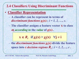
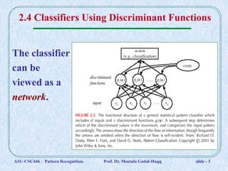
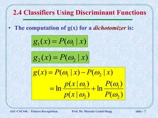
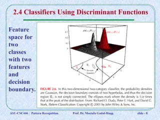
This document discusses Bayesian decision theory and classifiers that use discriminant functions. It covers several key topics: 1. Classifiers can be represented by discriminant functions gi(x) that assign vectors x to classes based on their values. The functions divide the space into decision regions. 2. Discriminant functions gi(x) are not unique and can be scaled or shifted without changing decisions. 3. Examples of discriminant functions include posterior probabilities P(ωi | x), likelihood functions P(x | ωi)P(ωi), and risk functions. 4. The two-category case uses a single discriminant function g(x) = g1(x) - g2

1. Chapter 2 (Part 2):
Bayesian Decision Theory
Prof. Dr. Mostafa Gadal-Haqq
Faculty of Computer & Information Sciences
Computer Science Department
AIN SHAMS UNIVERSITY
CSC446 : Pattern Recognition
(Study DHS-Chapter 2: Sec 2.4-2.6)
ASU-CSC446 : Pattern Recognition. Prof. Dr. Mostafa Gadal-Haqq slide - 1

2. 2.4 Classifiers Using Discriminant Functions
• Classifier Representation
– A classifier can be represent in terms of
discriminant functions gi(x) ; i = 1, 2, …, c.
– The classifier assigns a feature vector x to class
i according to the value of g(x) .
– the discriminant functions gi(x) divide the feature
space into c decision regions Ri ; i = 1, 2,…, c .
x  Ri if gi(x) > gj(x) j  i
ASU-CSC446 : Pattern Recognition. Prof. Dr. Mostafa Gadal-Haqq slide - 2

3. 2.4 Classifiers Using Discriminant Functions
The classifier
can be
viewed as a
network.
ASU-CSC446 : Pattern Recognition. Prof. Dr. Mostafa Gadal-Haqq slide - 3

4. 2.4 Classifiers Using Discriminant Functions
• Properties of g(x)
– The choice of g(x) is not unique.
• If g(x) is scaled or shifted by a positive constant, we
will have the same decision:
g2(x) = k * g1(x), and g2(x) = g1(x) + k ; k is constant
– g(x) can be replaced by f(g(x)), where f(.) is a
monotonically increasing function:
g2(x) = f( g1( x ) )
ASU-CSC446 : Pattern Recognition. Prof. Dr. Mostafa Gadal-Haqq slide - 4

5. • Examples of g(.):
– For minimum-error rate, we could choose g(.):
gi(x) = P(i | x)
gi(x) = P(x | i) P(i)
gi(x) =ln(gi(x)) = ln P(x | i) + ln P(i)
– For the general case with risks, we choose g(.):
gi(x) = - R(i | x)
2.4 Classifiers Using Discriminant Functions
ASU-CSC446 : Pattern Recognition. Prof. Dr. Mostafa Gadal-Haqq slide - 5

6. • The two-category case
– A classifier is called a “dichotomizer” if it has
two discriminant functions g1 and g2.
– The decision rule becomes:
– we can put g(x)  g1(x) – g2(x), then
2.4 Classifiers Using Discriminant Functions
Decide 1 if g1(x) > g2(x); Otherwise decide 2
Decide 1 if g (x) > 0; Otherwise decide 2
ASU-CSC446 : Pattern Recognition. Prof. Dr. Mostafa Gadal-Haqq slide - 6

7. • The computation of g(x) for a dichotomizer is:
)|()( 11 xPxg 
2.4 Classifiers Using Discriminant Functions
)(
)(
ln
)|(
)|(
ln
)|()|()(
2
1
2
1
21





P
P
xp
xp
xPxPxg


)|()( 22 xPxg 
ASU-CSC446 : Pattern Recognition. Prof. Dr. Mostafa Gadal-Haqq slide - 7

8. 2.4 Classifiers Using Discriminant Functions
Feature
space for
two
classes
with two
features
and
decision
boundary.
ASU-CSC446 : Pattern Recognition. Prof. Dr. Mostafa Gadal-Haqq slide - 8

9. 2.5 The Univariate Normal Density
• A density that is analytically tractable
• Continuous density
• A lot of processes are asymptotically
Gaussian
Where:
 = mean (or expected value) of x
2 = squared deviation or variance
,
2
1
exp
2
1
)(
2













 




x
xp



1)( dxxp
ASU-CSC446 : Pattern Recognition. Prof. Dr. Mostafa Gadal-Haqq slide - 9

10. 2.5 The Normal Density
• Multivariate Normal Density
– Multivariate normal density in d dimensions is:
where:
x = (x1, x2, …, xd)t = The multivariate random variable
 = (1, 2, …, d)t = the mean vector
 = d*d covariance matrix, || and -1 are it determinant
and inverse, respectively .






 
)x()x(
2
1
exp
)2(
1
)x( 1
2/12/


t
d
p
ASU-CSC446 : Pattern Recognition. Prof. Dr. Mostafa Gadal-Haqq slide - 10

11. 2.6 Discriminant Functions for the Normal Density
• The minimum-error-rate the discriminant functions:
gi(x) = ln p(x | i) + ln P(i)
• if the densities p(x|ωi) are multivariate normal, i.e.,
if p(x|ωi) ~ N(µi,Σi).
• In this case,
• Let us consider a number of special cases:
ASU-CSC446 : Pattern Recognition. Prof. Dr. Mostafa Gadal-Haqq slide - 11

12. 2.6 Discriminant Functions for the Normal Density
• Case 1: Σi = σ2I:
• when the features are statistically independent, and
when each feature has the same variance, σ2. In this
case:
Σi = σ2I, |Σi| = σ2d , and Σi
−1 = (1/σ2)I.
• The discriminant function is then:
• We ignored both |Σi| and the (d/2) ln 2π term, since they are
additive constants independent of i.
ASU-CSC446 : Pattern Recognition. Prof. Dr. Mostafa Gadal-Haqq slide - 12

13. 2.6 Discriminant Functions for the Normal Density
• where ||·|| is the Euclidean norm, that is,
||x − µi||2 = (x − µi)t (x − µi)
• Expansion ||x − µi
2|| yields
• Can be written as a linear discriminant functions:
• Where: and
ASU-CSC446 : Pattern Recognition. Prof. Dr. Mostafa Gadal-Haqq slide - 13

14. 2.6 Discriminant Functions for the Normal Density
• A classifier that uses linear discriminant functions
is called a linear machine.
ASU-CSC446 : Pattern Recognition. Prof. Dr. Mostafa Gadal-Haqq slide - 14

15. 2.6 Discriminant Functions for the Normal Density
• Reading:
– Case 2: Σi = Σ :
• the covariance matrices for all classes are
identical.
– Case 3: Σi = arbitrary:
• the general multivariate normal case, the
covariance matrices are different for each
category.
ASU-CSC446 : Pattern Recognition. Prof. Dr. Mostafa Gadal-Haqq slide - 15

16. 2.6 Discriminant Functions for the Normal Density
– Σi arbitrary:
ASU-CSC446 : Pattern Recognition. Prof. Dr. Mostafa Gadal-Haqq slide - 16

17. 2.6 Discriminant Functions for the Normal Density
• Numerical Example: (Two features, Two classes)







6
3
1







6
3
1








2
3
2







20
02/1
1







20
02
2







2/10
021
1







2/10
02/11
2
• using: P(w1)=P(w2)=0.5,
• The decision boundary g(x) = g1(x) - g2(x) =0
w1
w2
x2 - 3.514 + 1.125 x1 - 0.1875 x1
2=0
ASU-CSC446 : Pattern Recognition. Prof. Dr. Mostafa Gadal-Haqq slide - 17

18. Home Work (1)
• Write a report on Section 2.9: Bayesian Decision
theory - Discrete features.
• 2.9.1: Independent binary features
• Example 3: Bayesian Decisions for 3D binary Data
• Problem Exercises:
– Derive the decision boundary equation in the
previous example (slide #17).
ASU-CSC446 : Pattern Recognition. Prof. Dr. Mostafa Gadal-Haqq slide - 18