This document provides an overview of Bayesian classification. It begins by explaining that Bayesian classification is a statistical classifier that performs probabilistic predictions based on Bayes' theorem. It then provides an example of how a naive Bayesian classifier would work on a sample training dataset to classify whether someone buys a computer. The document concludes by discussing some advantages, such as being easy to implement and providing good results often, and disadvantages, such as the assumption of class conditional independence losing accuracy when dependencies exist among variables.

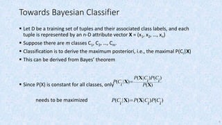
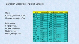
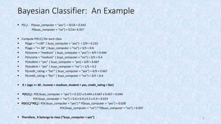
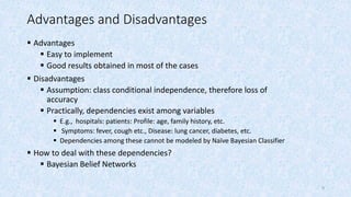
1. Bayesian Classification
MD. Zul Kawsar
1

2. Content
 Introduction
 Why We Use
 Example
 Advantage & Disadvantage
 Conclusion
2

3. 3
Bayesian Classification: Why?
 A statistical classifier: performs probabilistic prediction, i.e., predicts class
membership probabilities
 Foundation: Based on Bayes’ Theorem.
 Performance: A simple Bayesian classifier, naïve Bayesian classifier, has
comparable performance with decision tree and selected neural network
classifiers
 Incremental: Each training example can incrementally increase/decrease the
probability that a hypothesis is correct — prior knowledge can be combined with
observed data
 Standard: Even when Bayesian methods are computationally intractable, they can
provide a standard of optimal decision making against which other methods can
be measured

4. 4
Bayesian Theorem: Basics
 Let X be a data sample (“evidence”): class label is unknown
 Let H be a hypothesis that X belongs to class C
 Classification is to determine P(H|X), the probability that the hypothesis
holds given the observed data sample X
 P(H) (prior probability), the initial probability
 E.g., X will buy computer, regardless of age, income, …
 P(X): probability that sample data is observed
 P(X|H) (posteriori probability), the probability of observing the sample X,
given that the hypothesis holds
 E.g., Given that X will buy computer, the prob. that X is 31..40,
medium income

5. 5
Bayesian Theorem Cont..
 Given training data X, posteriori probability of a hypothesis H, P(H|X),
follows the Bayes theorem
 Informally, this can be written as
posteriori = likelihood x prior/evidence
 Predicts X belongs to C2 iff the probability P(Ci|X) is the highest among
all the P(Ck|X) for all the k classes
 Practical difficulty: require initial knowledge of many probabilities,
significant computational cost
)(
)()|()|(
X
XX
P
HPHPHP 

6. 6
Towards Bayesian Classifier
 Let D be a training set of tuples and their associated class labels, and each
tuple is represented by an n-D attribute vector X = (x1, x2, …, xn)
 Suppose there are m classes C1, C2, …, Cm.
 Classification is to derive the maximum posteriori, i.e., the maximal P(Ci|X)
 This can be derived from Bayes’ theorem
 Since P(X) is constant for all classes, only
needs to be maximized
)(
)()|(
)|(
X
X
X
P
i
CP
i
CP
i
CP 
)()|()|(
i
CP
i
CP
i
CP XX 

7. 7
Bayesian Classifier: Training Dataset
Class:
C1:buys_computer = ‘yes’
C2:buys_computer = ‘no’
Data sample
X = (age <=30,
Income = medium,
Student = yes
Credit_rating = Fair)
age income studentcredit_ratingbuys_computer
<=30 high no fair no
<=30 high no excellent no
31…40 high no fair yes
>40 medium no fair yes
>40 low yes fair yes
>40 low yes excellent no
31…40 low yes excellent yes
<=30 medium no fair no
<=30 low yes fair yes
>40 medium yes fair yes
<=30 medium yes excellent yes
31…40 medium no excellent yes
31…40 high yes fair yes
>40 medium no excellent no

8. 8
Bayesian Classifier: An Example
 P(Ci): P(buys_computer = “yes”) = 9/14 = 0.643
P(buys_computer = “no”) = 5/14= 0.357
 Compute P(X|Ci) for each class
 P(age = “<=30” | buys_computer = “yes”) = 2/9 = 0.222
 P(age = “<= 30” | buys_computer = “no”) = 3/5 = 0.6
 P(income = “medium” | buys_computer = “yes”) = 4/9 = 0.444
 P(income = “medium” | buys_computer = “no”) = 2/5 = 0.4
 P(student = “yes” | buys_computer = “yes) = 6/9 = 0.667
 P(student = “yes” | buys_computer = “no”) = 1/5 = 0.2
 P(credit_rating = “fair” | buys_computer = “yes”) = 6/9 = 0.667
 P(credit_rating = “fair” | buys_computer = “no”) = 2/5 = 0.4
 X = (age <= 30 , income = medium, student = yes, credit_rating = fair)
 P(X|Ci) : P(X|buys_computer = “yes”) = 0.222 x 0.444 x 0.667 x 0.667 = 0.044
 P(X|buys_computer = “no”) = 0.6 x 0.4 x 0.2 x 0.4 = 0.019
 P(X|Ci)*P(Ci) : P(X|buys_computer = “yes”) * P(buys_computer = “yes”) = 0.028
P(X|buys_computer = “no”) * P(buys_computer = “no”) = 0.007
 Therefore, X belongs to class (“buys_computer = yes”)

9. 9
Advantages and Disadvantages
 Advantages
 Easy to implement
 Good results obtained in most of the cases
 Disadvantages
 Assumption: class conditional independence, therefore loss of
accuracy
 Practically, dependencies exist among variables
 E.g., hospitals: patients: Profile: age, family history, etc.
 Symptoms: fever, cough etc., Disease: lung cancer, diabetes, etc.
 Dependencies among these cannot be modeled by Naïve Bayesian Classifier
 How to deal with these dependencies?
 Bayesian Belief Networks

10. Conclusion
 It is one of the oldest formal classification algorithms, and yet even in
its simplest form it is often surprisingly effective.
 It is widely used in areas such as text classification and spam filtering.
 It tremendously appealing because of its simplicity, elegance, and
robustness.
10

11. Thank You
11