Downloaded 55 times


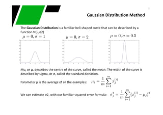
![16
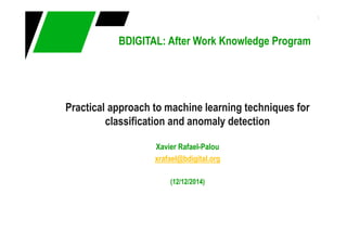
- We add new random variable x to the system for a better performance
x = size degree of the fruit [1,2,3…]
- So, we get probs of p(x) too
- Since x depends on the type of fruit, we get densities of x depending on the type of
fruit:
p(x| y=A) , p(x | y=M) “conditional probability densities”
How size affects our attitude regarding the type of fruit in question?
- p(y=A | x) = (p(x| y=A) P(y=A)) / p(x)
- P(y=M | x) = (p(x| y=M) P(y=M)) /p(x)
Naive Bayes: A if p(y=A | x) >= p(y=M | x) else M (probs “a posteriori”)
Probabilistic classifiers](https://image.slidesharecdn.com/intro-classification-anomalies-141220021327-conversion-gate01/85/Introduction-to-conventional-machine-learning-techniques-16-320.jpg)
![20
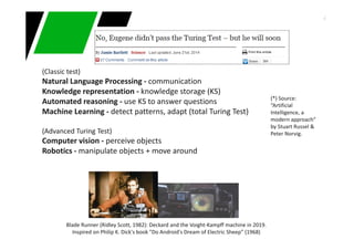
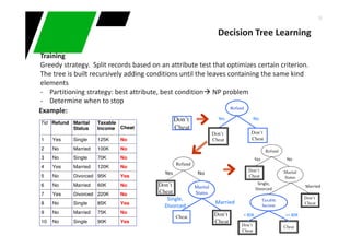
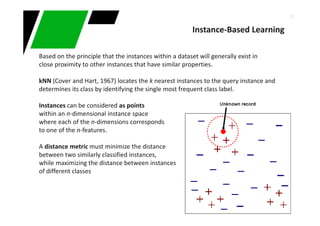
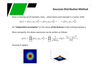
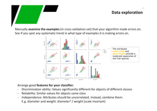
Partitioning strategy : Preferred aattribute's that generate disjoint sets (homogeneity)
Strategy examples :
∑−=
j
tjptGINI 2
)]|([1)(
Non-homogeneous,
High degree of impurity
Homogeneous,
Low degree of impurity
p( j | t) is the relative frequency of class j at node t
)|(max1)( tjPtError
j
−=
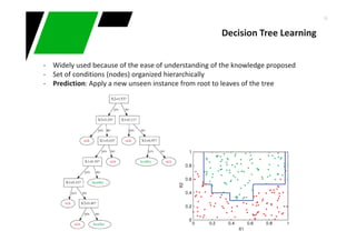
Decision Tree Learning
Measures homogeneity of a node. Used in CART, SLIQ, SPRINT
−= ∑
=
k
i
i
split
iEntropy
n
n
pEntropyGAIN 1
)()(
Measures misclassification error made by a node
Choose split that achieves most homogeneity reduction (e.g. ID3, C4.5)](https://image.slidesharecdn.com/intro-classification-anomalies-141220021327-conversion-gate01/85/Introduction-to-conventional-machine-learning-techniques-20-320.jpg)


![44
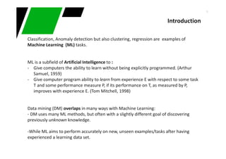
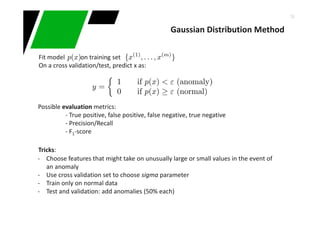
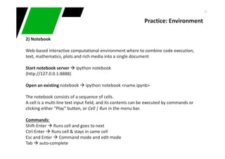
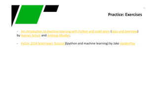
Practice: Environment
0) Python:
Language interpreted dynamically-typed nature
Download:
- Python already installed:
pip install ipython or only dependencies "ipython[notebook]“
- Otherwise:
Anaconda (http://continuum.io/downloads) is a completely free Python distribution
(including for commercial use and redistribution). It includes over 195 of the most
popular python packages for science, math, engineering, data analysis.
$ Conda info
$ conda install <packageName>
$ conda update <packageName>](https://image.slidesharecdn.com/intro-classification-anomalies-141220021327-conversion-gate01/85/Introduction-to-conventional-machine-learning-techniques-44-320.jpg)


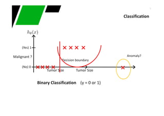
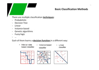
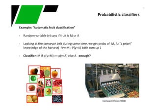
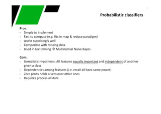
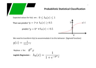
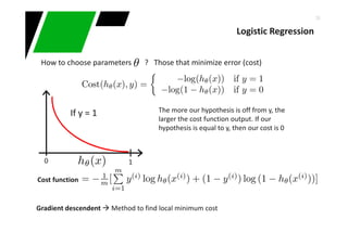
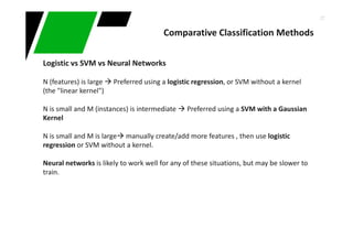
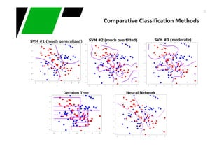
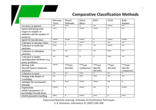
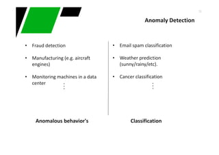
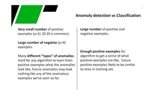
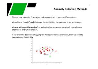
This document provides an overview of machine learning techniques for classification and anomaly detection. It begins with an introduction to machine learning and common tasks like classification, clustering, and anomaly detection. Basic classification techniques are then discussed, including probabilistic classifiers like Naive Bayes, decision trees, instance-based learning like k-nearest neighbors, and linear classifiers like logistic regression. The document provides examples and comparisons of these different methods. It concludes by discussing anomaly detection and how it differs from classification problems, noting challenges like having few positive examples of anomalies.


![[ppt]](https://cdn.slidesharecdn.com/ss_thumbnails/ppt2931-thumbnail.jpg?width=640&height=640&fit=bounds)
![[ppt]](https://cdn.slidesharecdn.com/ss_thumbnails/ppt3441-thumbnail.jpg?width=640&height=640&fit=bounds)


