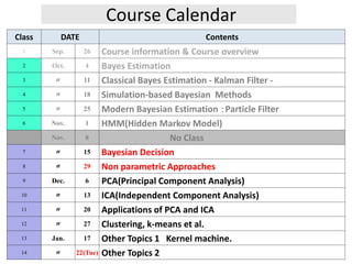
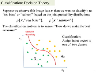
1. The document outlines the course calendar for a Bayesian estimation course, with topics including Bayes estimation, Kalman filters, particle filters, hidden Markov models, Bayesian decision theory, and applications of principal component analysis and independent component analysis. 2. The lecture on Bayesian decision theory introduces classification and decision problems, Bayes' decision theory, discriminant functions, and the Gaussian case. It discusses classifying observations to categories based on loss functions and conditional risk to minimize overall risk. 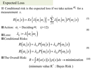3. Bayesian decision theory aims to assign observations to categories to minimize the expected loss. It considers prior probabilities, likelihood functions, posterior probabilities, and loss functions to derive decision rules that minimize risk or probability of error.

1. Course Calendar
Class DATE Contents
1 Sep. 26 Course information & Course overview
2 Oct. 4 Bayes Estimation
3 〃 11 Classical Bayes Estimation - Kalman Filter -
4 〃 18 Simulation-based Bayesian Methods
5 〃 25 Modern Bayesian Estimation ：Particle Filter
6 Nov. 1 HMM(Hidden Markov Model)
Nov. 8 No Class
7 〃 15 Bayesian Decision
8 〃 29 Non parametric Approaches
9 Dec. 6 PCA(Principal Component Analysis)
10 〃 13 ICA(Independent Component Analysis)
11 〃 20 Applications of PCA and ICA
12 〃 27 Clustering, k-means et al.
13 Jan. 17 Other Topics 1 Kernel machine.
14 〃 22(Tue) Other Topics 2

2. Lecture Plan
Bayes Decision
1. Introduction
1.1 Pattern Recognition-
1.2 An Example Classification/Decision Theory
2. Bayes Decision Theory
2.1 Decision using Posterior Probability
2.2 Decision by Minimizing Risk
3. Discriminate Function
4. Gaussian Case

3. 1. Introduction
3
1.1 Pattern Recognition
The second part of this course is concerned about Pattern Recognition.
Pattern recognitions (Machine Learning) want to give very high skills
for sensing and taking actions as humans do according to what they
observe.
Definitions of Pattern Recognition appeared in books
“The assignment of a physical object or event to one of several pre-
specified categories”
by Duda et al.[1]
“The science that concerns the description or classification
(recognition) of measurements”
by Schalkoff (Wiley Online Library)

4. Fish-Sorting Process
Sea bass 鱸
Salmon 鮭
R.O. Duda, P.E. Hart, and D. G. Stork,
“Pattern Classification”, John Wiley & Sons, 2nd edition, 2004

5.  
 
1
2
.
:
:feature vector in 2-d feature space
:
: action
"Correct dicision " should be an appropriate function of data
eg
x lightness
x width
x


 
  
 
x
x
x
1.2 An Example (Duda, Hart, & Stork 2004)
5
Automatic Fish-Sorting Process
action １
belt conveyer
action 2

6. Typical pattern Recognition issues:
■ Classification ■ Regression
■ Clustering ■ Dimension Reduction
(Visualization)
Pattern Recognition System
data
Measurement
Preprocessing
Dimension
Reduction
Feature
Selection
Recognition
Classification
Model
change
Evaluation
analysis
results
PCA (ICA)
Clustering Cross-
ValidationPDF estimation
PDF: Probability Density Function

7. 7
Classification/ Decision Theory
Suppose we observe fish image data x, then we want to classify it to
“sea bass” or “salmon” based on the joint probability distributions
The classification problem is to answer “How do we make the best
decision?”
   p ," sea bass" , p ," salmon"x x
x1
x2
Decision
Boundary
Classification:
Assign input vector to
one of two classes
R2
R1

8. Framework: - Two Category case (fish sorting example) -
■ State of nature (Class) ω (discrete random variable)
■ Prior Probability
■ Class-conditioned Probability (Likelihood)
Measurement x : brightness of fish (scalar continuous variable)
Class-conditional probability density function for each class:
1
2
: sea bass
: salmon
 
 


2. Bayes’ Decision Theory
   
   
1 2
1 2
,
where 1
P P
P P
 
  
   
   
1 1
2 2
PDF for given that the state of nature is
PDF for given that the state of nature is
p x x
p x x
 
 



9. 9
Fig. 1 Class-conditioned probabilities

10. 10
2.1 Decision Using Posterior Probability
■ Posterior Probabilities
■ Decision Rule (1) Minimizing error probability
■ Decision Rule (2) Likelihood ratio
   
 
   
 
the probability of being given that has been measuredDefine
Bayes rule derives
j
j j
j
xjP x
p x P
P x
p x
 
 



   
   
1 21
2 1 2
if >
if <
P x P x
P x P x
 
  
Decide
 
 
 
 
11 1
2 22
if
p x P
Pp x
 
 


Decide
independent of
observation x
(1)
(2)
(3)

11. 11
Fig. 2 Decision
(a) Posterior Probabilities
(b) Likelihood ratio

12. 12
Probability of Error
■ Error probability for a measurement x by decision
■ Average probability of error
   
 
        
               2 1 2 2 1 1
1 2 1 2
if we decide ( )2 1 1
if we decide ( )1 2 2
:
P x P x P x P P x P
P x x R
P x x R
P error xEx
p x dx p x dx dx dx
P error x p x dx
P error x
P error
     
 
 
 


 


     
R R R R
(4)
(5)
Fig. 3 P(error)

13. 13
2.2 Decision by Minimizing Risk
■ Alternate Bayes Decision based on risk which defines “how much
costly each action is ?”
Suppose we observe x then take action according to make a decision
(ωi) if the true state of nature is ωj , we introduce the loss function
■ Example of loss function
From a medical image we want to classify (determine) whether it
contains cancer tissues or not.
 i j  
i
1 2
1 2
cancer, normal,
cancer, normal
 
 
 
 
cancer normal
cancer 0 1
normal 100 0
 i j  
1
2
1 2
(6)
Loss Function

14. Expected Loss
■ Conditional risk is the expected loss if we take action for a
measurement x.
■Action: = Deciding (i=12)
■Loss:
■Conditional Risks:
■The Overall Risk:
        
2
1
:i i j i j j
j
R x Ex P x       

  
i
i i
 :ij i j   
     
     
1 11 1 12 2
2 21 1 22 2
R x P x P x
R x P x P x
    
    
 
 
    
*
minimization
(minmum value R : Bayes Risk )
R R x x p x dx 
(7)
(8)
(9)
(10)

15. 15
Minimum Risk Decision Rule (1)
   
   
1 21
2 1 2
if <
if >
R x R x
R x R x
 
  
Decide
   
       
1 2
21 11 1 12 22 2
Here , <
>
R x R x
P x P x
 
       
Minimum Risk Decision Rule (2)
 
 
 
 
 
 
1
1 12 22 2
21 11 12
2
if
Otherwise decide
threshold
P x P
PP x

   
  




Decide
(11)
(12)
(13)

16. 16
Fig. 4 Likelihood ratio

17. 17
Minimum error probability decision
=Minimizing the risk with zero-one loss function
Zero-One Loss Function:
 
 
 
 
1 2
12
Likekihood ratio decision rule (13) becomes
minimum error decision
P x P
PP x
 




Zero-One Loss Function:
 
0 if 0 1
,
1 if 1 0
i j ij
i j
i j
   
  
       
(14)
(15)

18. General Framework:
■ Finite set of states of nature (c Classes) :
■ Actions :
■ Loss:
■ Measurement:
 1 2, , c  
Generalization
: d-dimensional vector (feature vector)x
 1 2, , a  
     : 1,..., 1,...,ij i j i a j c     

19. 19
3. Discriminant Function
19
Classifiers represented by discriminant functions : gi(x) i=1,…c
max gi(x)
g1(x) g2(x) gc(x)
x2
…
 where arg max
i
j
j
i g

 x
   Classifier minimizing the conditional risk: =i ig x R x
       
     
Minimizing error probability: =
Alternate function: =ln ln
i i i i
i i i
g x P x p x P
g x p x P
  
 


xdx1 …input
discriminant
fnctions
Classifier
Network structure
action

20. 2020
■ Single discriminant function:
Two-category case
 
 
   
1
2
1 2
if 0
if 0
gives the decision boundary
g x
g x
g x g x





Decide
4．Gaussian Case:
   
     
     1
Multivariate Gaussian: ,
=ln ln
1 1
ln2 ln ln
2 2 2
i i i
i i i
T
i i i i i
p
g x p x P
d
x x P

 
 


      
x  
   
(17 )
(18)
(16)     1 2=g x g x g x

21. 21
       
 
1
1 1 1
1 1
= ln2 ln ln
2 2 2
1 1 1
ln ln
2 2 2
T
i i i i i i
T T T
i i i i i i i i
d
g x x x P
x x x P
 


  
     
     
   
      
  0= T
i i i ig x x  T
x W x
 1
0
1 1
ln ln
2 2
T
i i i i i iP 
      
Case (i=1,2)
Boundary is given by a linear line
i   1 2General Case
Boundary is quadratic curves
 
decision
boundary
decision
boundary
(19)
(20)
1 11
where ,
2
i i i i i 
  W   

22. 22
References:
1) R.O. Duda, P.E. Hart, and D. G. Stork, “Pattern Classification”,
John Wiley & Sons, 2nd edition, 2004
2) C. M. Bishop, “Pattern Recognition and Machine Learning”,
Springer, 2006
3) E. Alpaydin, Introduction to Machine Learning, MIT Press, 2009
4) A. Huvarinen et. al., ”Independent Component Analysis”
Wiley-Interscience 2001
Another action : Rejection
No classification for lower degree of conviction case
What next ?
In the discussions so far all of the relevant probabilities are known,
but this assumption will not be assured.
Fukunaga’s definition of Pattern Recognition:
“A problem of estimating density functions in a high–dimensional
space and dividing the space into the regions of categories or
classes”

23. 23
 
 
   
 
 
     
1
/2 1/2
1
1 1 1
, exp
22
is d-dimensional random vector
:
: :
: Determinant of
T
d
T
d
x x
x x x
E x
Cov x E x x
  


 
 
      
 

   
  
Appendix:
Multivariable Gaussian Density Distribution