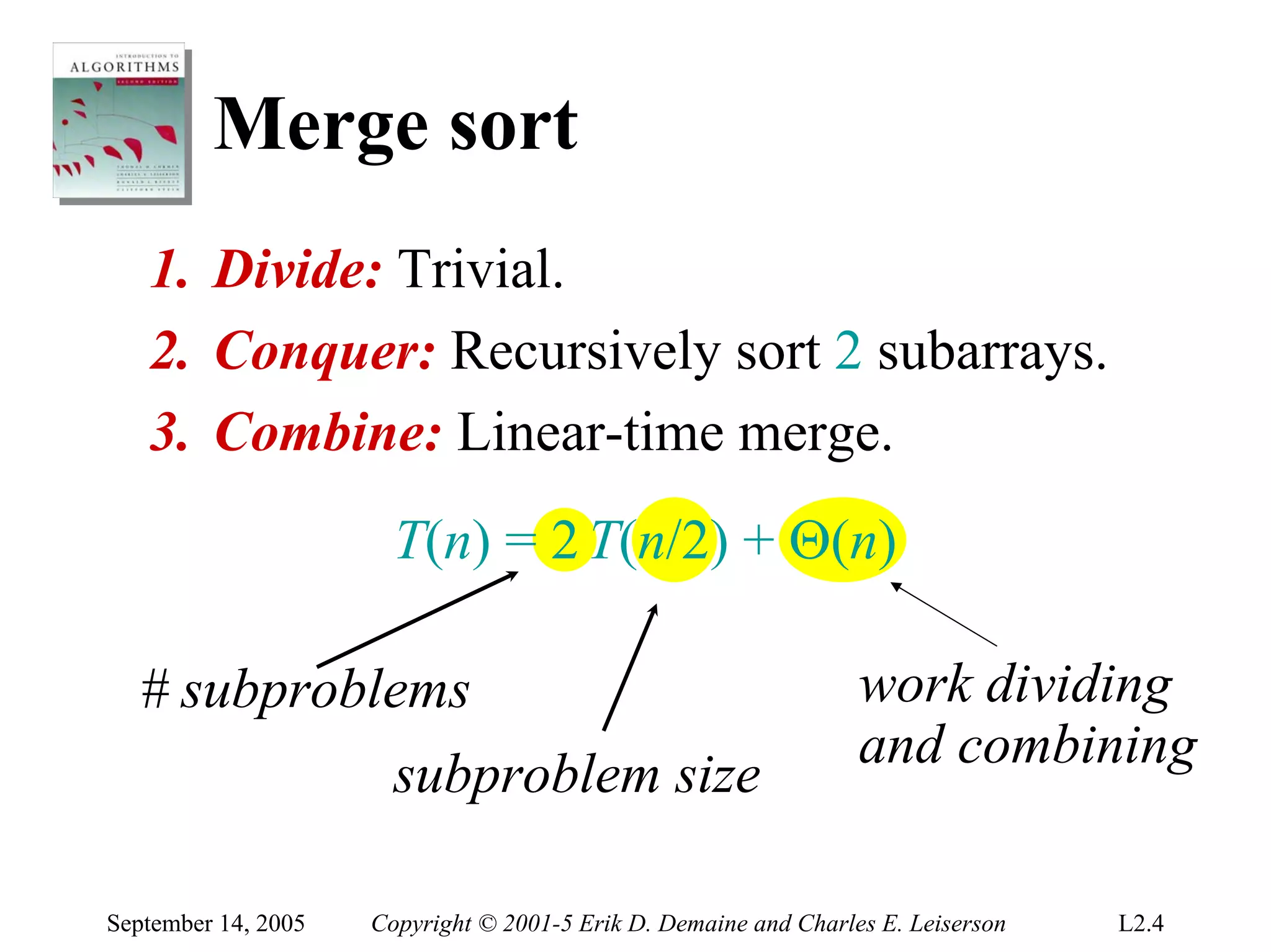
The document discusses the divide-and-conquer algorithm design paradigm and several examples that use this paradigm. It begins by outlining the three main steps of divide-and-conquer: 1) divide the problem into subproblems, 2) conquer the subproblems recursively, and 3) combine the subproblem solutions. It then provides examples that use divide-and-conquer, including merge sort, binary search, powering a number, computing Fibonacci numbers, and matrix multiplication. For each example, it describes how the problem is divided and conquered recursively and analyzes the running time.

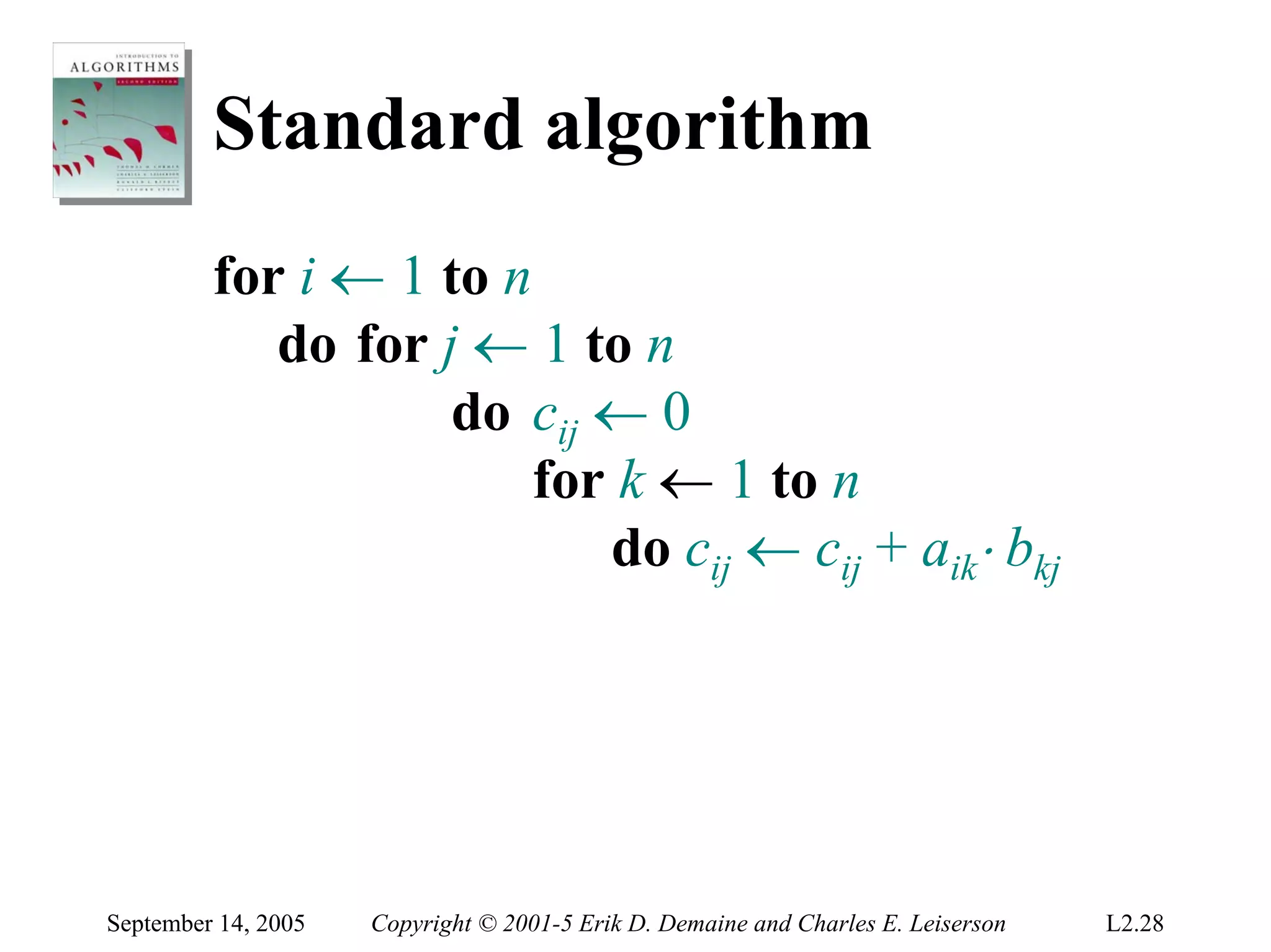
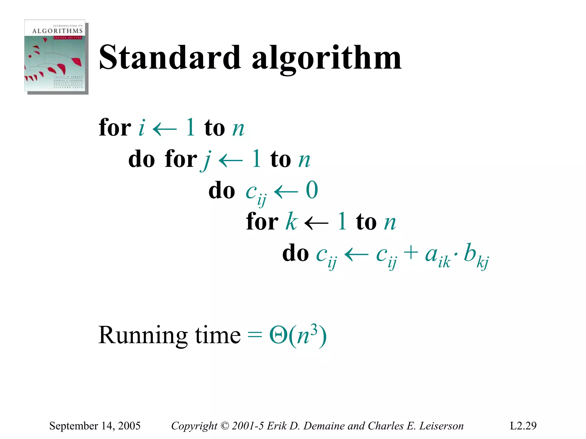
![Matrix multiplication
Input: A = [aij], B = [bij].
i, j = 1, 2,… , n.
Output: C = [cij] = A⋅ B.
⎡ c11 c12 L c1n ⎤ ⎡ a11 a12 L a1n ⎤ ⎡ b11 b12 L b1n ⎤
⎢c c L c2 n ⎥ ⎢a21 a22 L a2 n ⎥ ⎢b21 b22 L b2 n ⎥
⎢ 21 22 ⎥=⎢ ⎥⋅⎢ ⎥
⎢ M M O M ⎥ ⎢ M M O M ⎥ ⎢ M M O M ⎥
⎢c c L cnn ⎥ ⎣ an1 an 2
⎢ L ann ⎥ ⎢bn1 bn 2 L bnn ⎥
⎣ n1 n 2 ⎦ ⎦ ⎣ ⎦
n
cij = ∑ aik ⋅ bkj
k =1
September 14, 2005 Copyright © 2001-5 Erik D. Demaine and Charles E. Leiserson L2.27](https://image.slidesharecdn.com/lec3-algott-100204073334-phpapp02/75/Lec3-Algott-27-2048.jpg)