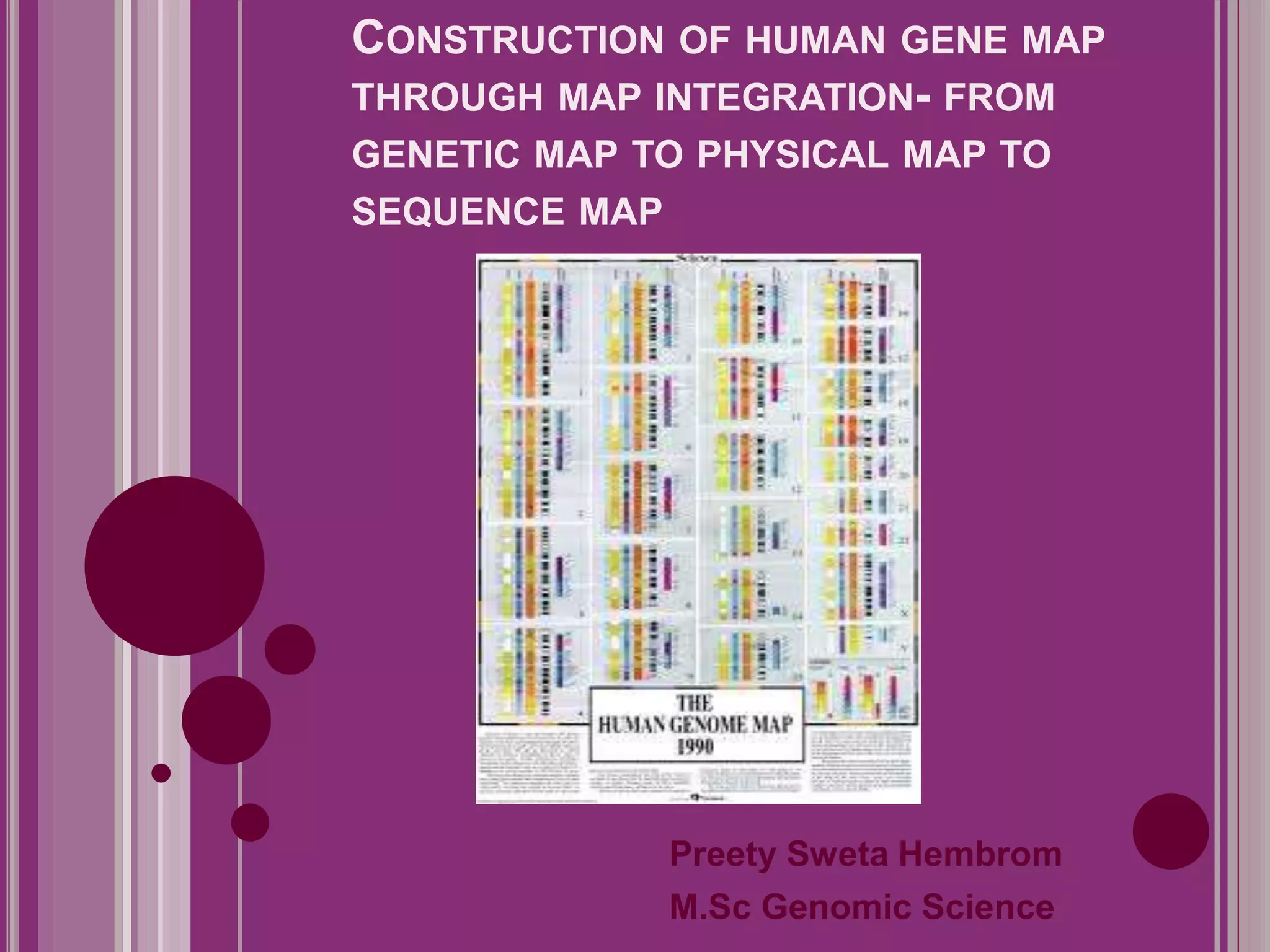
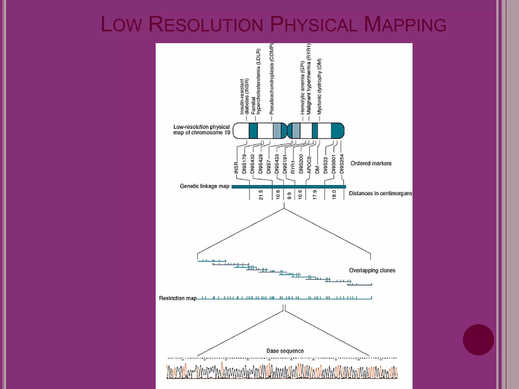
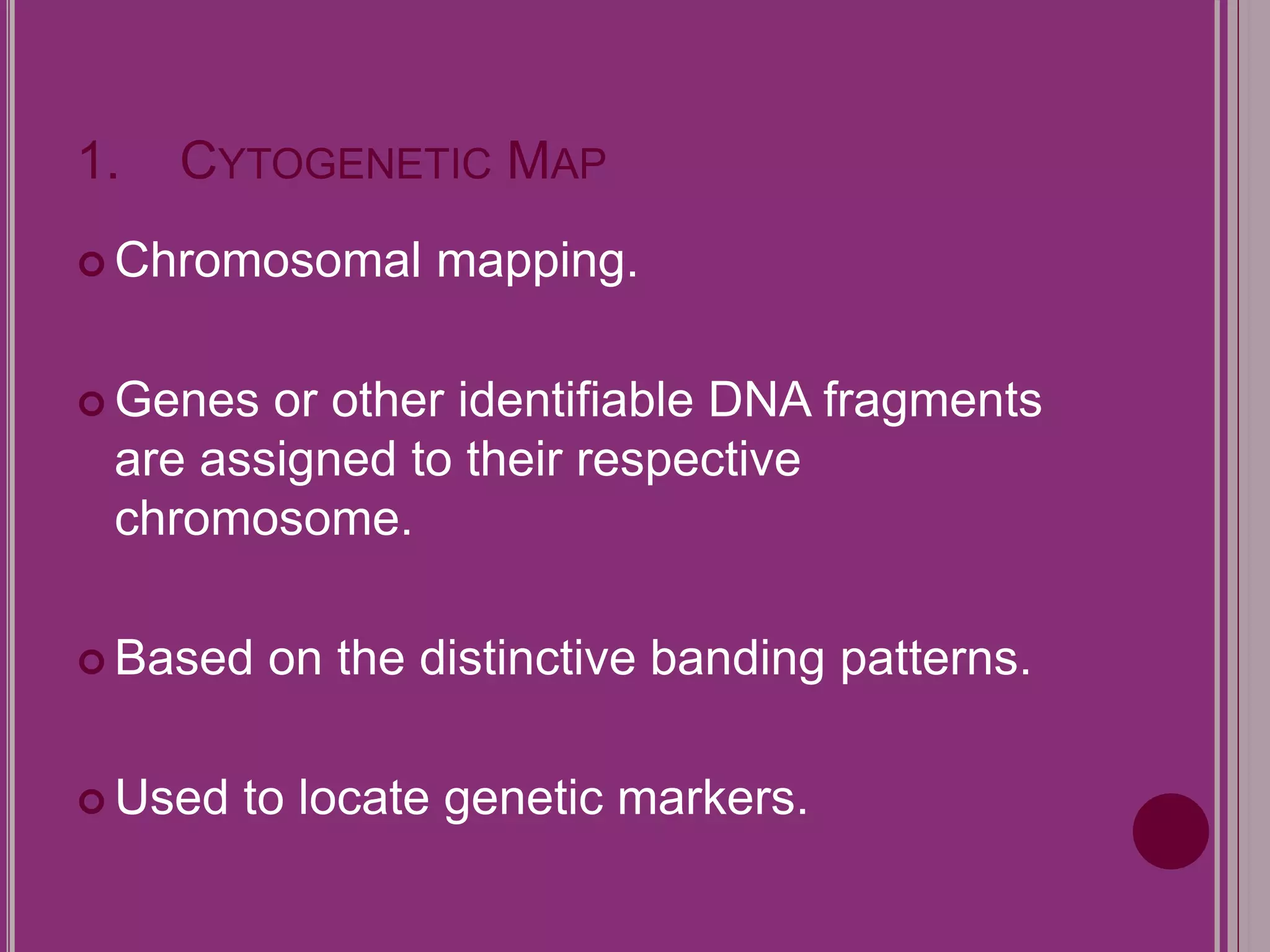
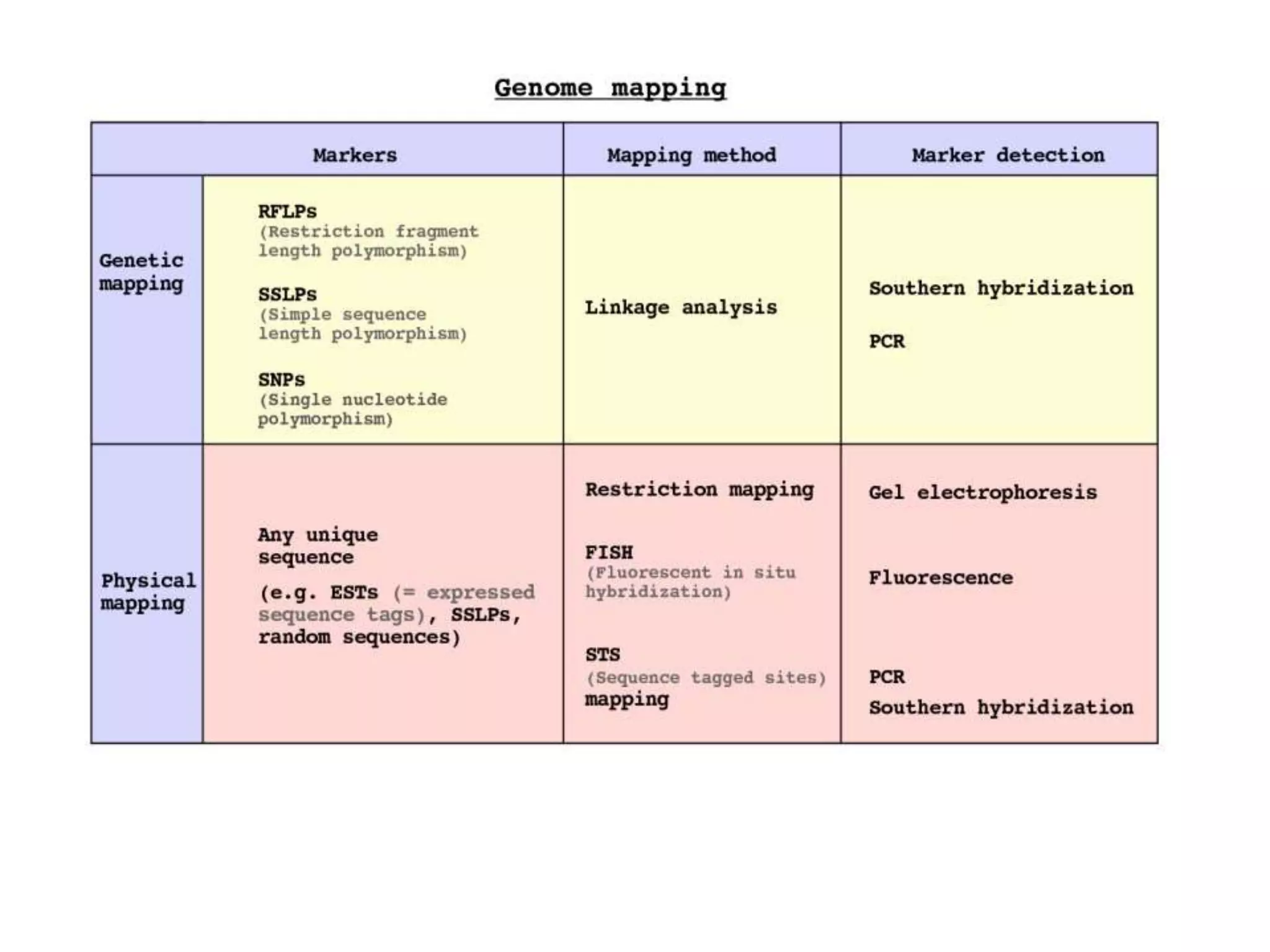
The document outlines the construction of a human gene map using integration from genetic maps to physical maps and sequence maps, focusing on various DNA markers such as RFLPs, SSLPs, and SNPs. It describes the methods used to measure genetic linkage and physical distances on chromosomes, highlighting the importance of technologies like FISH and sequencing methods such as the clone contig and whole genome shotgun approaches. The ultimate goal is to fully sequence the human genome to aid in understanding genes and developing treatments for diseases.

1. CONSTRUCTION OF HUMAN GENE MAP
THROUGH MAP INTEGRATION- FROM
GENETIC MAP TO PHYSICAL MAP TO
SEQUENCE MAP
Preety Sweta Hembrom
M.Sc Genomic Science

2. MAP INTEGRATION
Mapping is identifying relationships between
genes on chromosomes
Two broad categories of map:
1. Genetic map
2. Physical map

3. GENETIC MAP
 Describes the order of genes or other markers
and the spacing between them on each
chromosome.
 Use of genetic markers.
 DNA based marker can also serve as markers.
 Value of genetic map is that an inherited
disease can be located on the map.
 Used to find the exact location of several
important disease genes.

4. DNA MARKER

5. 1. RFLPS (RESTRICTION FRAGMENT LENGTH
POLYMORPHISMS):
 Defined by the presence or absence of a
specific site- restriction site.
 If 2 related but different DNA molecules are
cut with the same restriction enzymes, a
segment of different lengths are produced.
 And RFLP is the difference between two
DNA sequences that affect a restriction site.

7. 2. SIMPLE SEQUENCE LENGTH
POLYMORPHISMS (SSLPS)
 Arrays of repeat sequences that display length
variations, different alleles containing different
numbers of repeat units.
 Two types of SSLP:
I. Minisatellites:-
 Also known as variable number of tandem
repeats (VNTRs)
 Defined by the presence of a nucleotide
sequence that is repeated several times.

8. II. MICROSATELLITES
 simple tandem repeats (STRs)
 Whose repeats are shorter, usually dinucleotide or
tetra nucleotide units.
 Polymorphic because the number of repeats may
vary.
 Scored by determining their length by PCR.
 Fragments are separated by electrophoresis.
 Primers is labeled with fluorescent dye.
 Human genome contains 5870 markers.

9. 3. SNPS (SINGLE NUCLEOTIDE
POLYMORPHISMS)
Positions in a genome where some
individuals have one nucleotide and others
have a different nucleotide.
Some of which also give rise to RFLPs.
 In the human genome there are at least
1.42 million SNPs, only 100 000 of which
result in an RFLP.

10. LOD SCORE METHOD FOR ESTIMATING
RECOMBINATION FREQUENCY
 Imperfect pedigrees are analyzed statistically, using
a measure called the lod score (Morton, 1955).
 This stands for logarithm of the odds that the genes
are linked and is used primarily to determine if the
two markers being studied lie on the same
chromosome.
 If the LOD analysis establishes linkage then it can
also provide a measure of the most likely
recombination frequency.

11. THE LOD SCORE
 Computerized LOD score analysis is a simple way to
analyze complex family pedigrees in order to determine
the linkage between a trait and a marker, or two
markers.
 The method briefly, works as follows:
 Establish a pedigree
 Make a number of estimates of recombination frequency
 Calculate a LOD score for each estimate
 The estimate with the highest LOD score will be
considered the best estimate.

12. LOD SCORE
 The LOD score is calculated as follows:
 LOD = Z =Log10 probability of birth sequence with a given linkage
probability of birth sequence with no linkage
 By convention, a LOD score greater than 3.0 is considered
evidence for linkage.
 On the other hand, a LOD score less than -2.0 is considered
evidence to exclude linkage.

13. GENETIC MAP AS A FRAMEWORK FOR
PHYSICAL MAP CONSTRUCTION:

14. PHYSICAL MAP
 Determination of physical distance between
two points on chromosome.
 Distance in base pairs
Example: between physical marker and a
gene.
 Need overlapping fragments of DNA
 Requires vectors that accommodate large inserts
Examples: cosmids, YACs, and BACs

16. CONTD.
 Divided into 2 groups:
 Low Resolution Physical mapping:
i. Cytogenetic map
ii. cDNA map
iii. Contig map
 High Resolution Physical mapping:
i. Macrorestriction map
ii. RH mapping
iii. Sequence map

17. LOW RESOLUTION PHYSICAL MAPPING

18. 1. CYTOGENETIC MAP
 Chromosomal mapping.
Genes or other identifiable DNA fragments
are assigned to their respective
chromosome.
 Based on the distinctive banding patterns.
 Used to locate genetic markers.

20. 2. CDNA MAP
 Shows the position of expressed DNA
regions.
 Synthesized in the laboratory using mRNA
as a template.
 Can be mapped to genomic regions.
 Provide the chromosomal location of the
genes whose functions are currently
unknown.

21. 3. CONTIG MAPS
 Bottom up mapping.
 Involves cutting the chromosome into small pieces.
 Can be verified by FISH which localizes cosmids to
specific regions within chromosomal bands.
 Consist of a linked library of small overlapping
clones.

22. FLUORESCENT IN SITU HYBRIDIZATION (FISH)
 FISH is an optical mapping.
 FISH enables the position of a marker on a
chromosome or extended DNA molecule to be
directly visualized.
 In optical mapping the marker is a restriction site
and it is visualized as a gap in an extended DNA
fiber.
 In FISH, the marker is a DNA sequence that is
visualized by hybridization with a fluorescent probe.

23. FLUORESCENT IN SITU HYBRIDIZATION

24. HIGH RESOLUTION PHYSICAL MAPPING

25. 1. MACRORESTRICTION MAPS
 Single chromosome is cut into large pieces.
 Depicts the order of and distance between
sites at which rare- cutter enzymes cleave.
 Simplest way to construct is to compare the
fragment sizes.
 The scale of restriction mapping limited by
the sizes of the restriction fragments.

27. 2. RADIATION HYBRID MAPPING
 Shows an estimated distance between genetic
markers.
 A scientist exposes DNA to measure doses of
radiation.
 Useful for ordering markers in regions where highly
polymorphic genetic markers are scarce.
 Bridge between linkage map and sequence maps.

29. 3. SEQUENCE MAPPING
 Sequence tagged site (STS) mapping.
 Short sequence of DNA.
 Exact location and order of the bases of
sequence must be known.
May occur only once in the chromosome.

31. COMMON SOURCES OF STS

32. I. EXPRESSED SEQUENCE TAGS(ESTS)
 Obtained by analysis of cDNA clones.
cDNA is prepared by converting mRNA into
double stranded DNA.
 Thought to represent the sequences of the
genes being expressed.

34. II. SIMPLE SEQUENCE LENGTH
POLYMORPHISMS(SSLPS)
• Most genomes contain repeats of three or
four nucleotides
• Length of repeat varies due to slippage in
replication
• Use PCR with primers external to the repeat
region
• On gel, see difference in length of amplified
fragment

36. NEED TO INTEGRATE PHYSICAL AND GENETIC
MAPS:
 STS based mapping has its limitations.
 DNA fragments may lost or mistakenly mapped to a
wrong position.
 DNA fragment may become contaminated with host
genetic material.
 Comparing and integrating STS based physical
maps with genetic, RH, cytogenic maps.

37. CONTD
 Ultimate objective of human genome was to
complete DNA sequence for the organism.
 In order to locate genes and other interesting
features.
 So in order to master sequence of chromosome
involves several sequencing method:
1. Sequence assembly by clone Contig method.
2. Whole genome Shotgun sequencing.

38. 1. SEQUENCE ASSEMBLY BY THE CLONE
CONTIG METHOD:
 Conventional method for obtaining sequence of a
eukaryotic genome.
 Genomes are broken into fragments of upto 1.5 Mb
in length.
 Built up by identifying clones containing overlapping
fragments.

39. 2. WHOLE GENOME SHOTGUN SEQUENCING
 Uses a map to aid assembly of the master
sequence
 Used to speed up the acquisition of contig
sequence data for large genomes such as human
genome.
 At least two libraries are used.

40. MAPPING PHASE OF THE HUMAN GENOME
PROJECT
 Discovery of RFLPs.
 In 1987 first human RFLP map was published.
 Goal was a genetic map with density of one marker
per 1 Mb.
 The 1994 map contained 5800 markers of which
over 4000 were SSLPs.

42. SEQUENCING THE HUMAN GENOME
 The whole genome shotgun was first proposed as
an alternative to contig method.
 The first draft sequence of an entire human
chromosome (22) was published in December
1991.
 Finally on June 26, 2000 Francis Collins and Craig
Venter jointly announced the completion of project.

43. HUMAN GENOME
 Contains about 20,000 to 30,000 genes.
 Only 1-2% is coding region.
 Rest are “junk DNA”.
 Some sections of the human genome have a
sequence almost exactly the same as equivalent
sections in other vertebrates .

44. FUTURE OF THE HUMAN GENOME PROJECT
 Completion of a finished sequence is not only the
goal.
 Use of comparative genomics.
 Direct development of new drugs and therapies
against cancer and other diseases.