ss

1. Decision
trees
Lecture
11
David
Sontag
New
York
University
Slides adapted from Luke Zettlemoyer, Carlos Guestrin, and
Andrew Moore

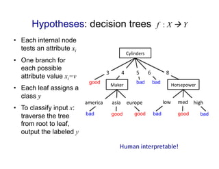
2. Hypotheses: decision trees f : X ! Y
• Each internal node
tests an attribute xi
• One branch for
each possible
attribute value xi=v
• Each leaf assigns a
class y
• To classify input x:
traverse the tree
from root to leaf,
output the labeled y
Cylinders
3
4
5
6
8
good bad bad
Maker
Horsepower
low
med
high
america
asia
europe
bad bad
good
good good
bad
Human
interpretable!

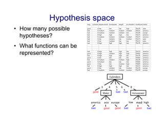
3. Hypothesis space
• How many possible
hypotheses?
• What functions can be
represented?
Cylinders
3
4
5
6
8
good bad bad
Maker
Horsepower
low
med
high
america
asia
europe
bad bad
good
good good
bad

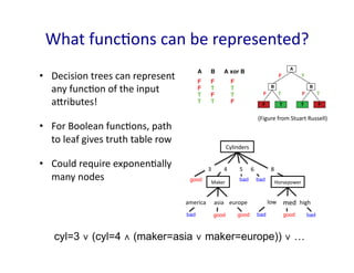
4. What
funcGons
can
be
represented?
• Decision
trees
can
represent
any
funcGon
of
the
input
aIributes!
• For
Boolean
funcGons,
path
to
leaf
gives
truth
table
row
• Could
require
exponenGally
many
nodes
Expressiveness
Discrete-input, discrete-output case:
– Decision trees can express any function of the input attribu
– E.g., for Boolean functions, truth table row path to leaf
F
T
A
B
F T
B
A B A xor B
F F F
F T T
T F T
T T F
F
F F
T
T T
Continuous-input, continuous-output case:
– Can approximate any function arbitrarily closely
Trivially, there is a consistent decision tree for any training set
w/ one path to leaf for each example (unless f nondeterministic
but it probably won’t generalize to new examples
Need some kind of regularization to ensure more compact deci
CS194-10 F
(Figure
from
Stuart
Russell)
cyl=3 ∨ (cyl=4 ∧ (maker=asia ∨ maker=europe)) ∨ …
Cylinders
3
4
5
6
8
good bad bad
Maker
Horsepower
low
med
high
america
asia
europe
bad bad
good
good good
bad

5. Learning
simplest
decision
tree
is
NP-­‐hard
• Learning
the
simplest
(smallest)
decision
tree
is
an
NP-­‐complete
problem
[Hyafil
&
Rivest
’76]
• Resort
to
a
greedy
heurisGc:
– Start
from
empty
decision
tree
– Split
on
next
best
a1ribute
(feature)
– Recurse

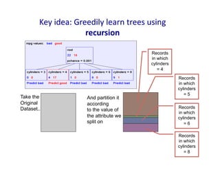
6. Key
idea:
Greedily
learn
trees
using
recursion
Take the
Original
Dataset..
And partition it
according
to the value of
the attribute we
split on
Records
in which
cylinders
= 4
Records
in which
cylinders
= 5
Records
in which
cylinders
= 6
Records
in which
cylinders
= 8

7. Recursive
Step
Records in
which cylinders
= 4
Records in
which cylinders
= 5
Records in
which cylinders
= 6
Records in
which cylinders
= 8
Build tree from
These records..
Build tree from
These records..
Build tree from
These records..
Build tree from
These records..

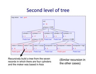
8. Second
level
of
tree
Recursively build a tree from the seven
records in which there are four cylinders
and the maker was based in Asia
(Similar recursion in
the other cases)

9. A full tree

10. Spli^ng:
choosing
a
good
aIribute
X1 X2 Y
T T T
T F T
T T T
T F T
F T T
F F F
F T F
F F F
X1
Y=t : 4
Y=f : 0
t f
Y=t : 1
Y=f : 3
X2
Y=t : 3
Y=f : 1
t f
Y=t : 2
Y=f : 2
Would we prefer to split on X1 or X2?
Idea: use counts at leaves to define
probability distributions, so we can
measure uncertainty!

11. Measuring
uncertainty
• Good
split
if
we
are
more
certain
about
classificaGon
a_er
split
– DeterminisGc
good
(all
true
or
all
false)
– Uniform
distribuGon
bad
– What
about
distribuGons
in
between?
P(Y=A) = 1/4 P(Y=B) = 1/4 P(Y=C) = 1/4 P(Y=D) = 1/4
P(Y=A) = 1/2 P(Y=B) = 1/4 P(Y=C) = 1/8 P(Y=D) = 1/8

12. Entropy
Entropy
H(Y)
of
a
random
variable
Y
More uncertainty, more entropy!
Information Theory interpretation:
H(Y) is the expected number of bits
needed to encode a randomly
drawn value of Y (under most
efficient code)
Probability
of
heads
Entropy
Entropy
of
a
coin
flip

13. High,
Low
Entropy
• “High
Entropy”
– Y
is
from
a
uniform
like
distribuGon
– Flat
histogram
– Values
sampled
from
it
are
less
predictable
• “Low
Entropy”
– Y
is
from
a
varied
(peaks
and
valleys)
distribuGon
– Histogram
has
many
lows
and
highs
– Values
sampled
from
it
are
more
predictable
(Slide from Vibhav Gogate)

14. Entropy
Example
X1 X2 Y
T T T
T F T
T T T
T F T
F T T
F F F
P(Y=t) = 5/6
P(Y=f) = 1/6
H(Y) = - 5/6 log2 5/6 - 1/6 log2 1/6
= 0.65
Probability
of
heads
Entropy
Entropy
of
a
coin
flip

15. CondiGonal
Entropy
CondiGonal
Entropy
H(Y |X)
of
a
random
variable
Y
condiGoned
on
a
random
variable
X
X1
Y=t : 4
Y=f : 0
t f
Y=t : 1
Y=f : 1
P(X1=t) = 4/6
P(X1=f) = 2/6
X1 X2 Y
T T T
T F T
T T T
T F T
F T T
F F F
Example:
H(Y|X1) = - 4/6 (1 log2 1 + 0 log2 0)
- 2/6 (1/2 log2 1/2 + 1/2 log2 1/2)
= 2/6

16. InformaGon
gain
• Decrease
in
entropy
(uncertainty)
a_er
spli^ng
X1 X2 Y
T T T
T F T
T T T
T F T
F T T
F F F
In our running example:
IG(X1) = H(Y) – H(Y|X1)
= 0.65 – 0.33
IG(X1) > 0 ! we prefer the split!

17. Learning
decision
trees
• Start
from
empty
decision
tree
• Split
on
next
best
a1ribute
(feature)
– Use,
for
example,
informaGon
gain
to
select
aIribute:
• Recurse

18. When
to
stop?
First split looks good! But, when do we stop?

19. Base Case
One
Don’t split a
node if all
matching
records have
the same
output value

20. Base Case
Two
Don’t split a
node if data
points are
identical on
remaining
attributes

21. Base
Cases:
An
idea
• Base
Case
One:
If
all
records
in
current
data
subset
have
the
same
output
then
don’t
recurse
• Base
Case
Two:
If
all
records
have
exactly
the
same
set
of
input
aIributes
then
don’t
recurse
Proposed Base Case 3:
If all attributes have small
information gain then don’t
recurse
•This is not a good idea

22. The
problem
with
proposed
case
3
y = a XOR b
The information gains:

23. If
we
omit
proposed
case
3:
y = a XOR b
The resulting decision tree:
Instead, perform
pruning after building a
tree

24. Decision
trees
will
overfit

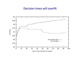
25. Decision
trees
will
overfit
• Standard
decision
trees
have
no
learning
bias
– Training
set
error
is
always
zero!
• (If
there
is
no
label
noise)
– Lots
of
variance
– Must
introduce
some
bias
towards
simpler
trees
• Many
strategies
for
picking
simpler
trees
– Fixed
depth
– Minimum
number
of
samples
per
leaf
• Random
forests

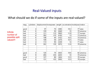
26. Real-­‐Valued
inputs
What
should
we
do
if
some
of
the
inputs
are
real-­‐valued?
Infinite
number of
possible split
values!!!

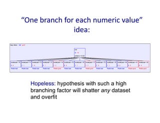
27. “One
branch
for
each
numeric
value”
idea:
Hopeless: hypothesis with such a high
branching factor will shatter any dataset
and overfit

28. Threshold
splits
• Binary
tree:
split
on
aIribute
X
at
value
t
– One
branch:
X
<
t
– Other
branch:
X
≥
t
Year
<78
≥78
good
bad
• Requires small change
• Allow repeated splits on same
variable along a path
Year
<70
≥70
good
bad

29. The
set
of
possible
thresholds
• Binary
tree,
split
on
aIribute
X
– One
branch:
X
<
t
– Other
branch:
X
≥
t
• Search
through
possible
values
of
t
– Seems
hard!!!
• But
only
a
finite
number
of
t’s
are
important:
– Sort
data
according
to
X
into
{x1,…,xm}
– Consider
split
points
of
the
form
xi
+
(xi+1
–
xi)/2
– Morever,
only
splits
between
examples
of
different
classes
maIer!
(Figures
from
Stuart
Russell)
Optimal splits for continuous attributes
Infinitely many possible split points c to define node test Xj > c ?
No! Moving split point along the empty space between two observed values
has no effect on information gain or empirical loss; so just use midpoint
Xj
c1
c2
Moreover, only splits between examples from different classes
can be optimal for information gain or empirical loss reduction
Xj
c2
c1
t1 t2
Optimal splits for continuous attributes
Infinitely many possible split points c to define node test Xj > c ?
No! Moving split point along the empty space between two observed values
has no effect on information gain or empirical loss; so just use midpoint
Xj
c1
c2
Moreover, only splits between examples from different classes
can be optimal for information gain or empirical loss reduction
Xj
c2
c1
t1 t2

30. Picking
the
best
threshold
• Suppose
X
is
real
valued
with
threshold
t
• Want
IG(Y
|
X:t),
the
informaGon
gain
for
Y
when
tesGng
if
X
is
greater
than
or
less
than
t
• Define:
• H(Y|X:t)
=
p(X
<
t)
H(Y|X
<
t)
+
p(X
>=
t)
H(Y|X
>=
t)
• IG(Y|X:t)
=
H(Y)
-­‐
H(Y|X:t)
• IG*(Y|X)
=
maxt
IG(Y|X:t)
• Use:
IG*(Y|X)
for
conGnuous
variables

31. What
you
need
to
know
about
decision
trees
• Decision
trees
are
one
of
the
most
popular
ML
tools
– Easy
to
understand,
implement,
and
use
– ComputaGonally
cheap
(to
solve
heurisGcally)
• InformaGon
gain
to
select
aIributes
(ID3,
C4.5,…)
• Presented
for
classificaGon,
can
be
used
for
regression
and
density
esGmaGon
too
• Decision
trees
will
overfit!!!
– Must
use
tricks
to
find
“simple
trees”,
e.g.,
• Fixed
depth/Early
stopping
• Pruning
– Or,
use
ensembles
of
different
trees
(random
forests)

32. Ensemble
learning
Slides adapted from Navneet Goyal, Tan, Steinbach,
Kumar, Vibhav Gogate

33. Ensemble
methods
Machine learning competition with a $1 million prize

34. Bias/Variance
Tradeoff
Hastie, Tibshirani, Friedman “Elements of Statistical Learning” 2001

35. Reduce
Variance
Without
Increasing
Bias
• Averaging
reduces
variance:
Average models to reduce model variance
One problem:
only one training set
where do multiple models come from?
(when predictions
are independent)

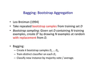
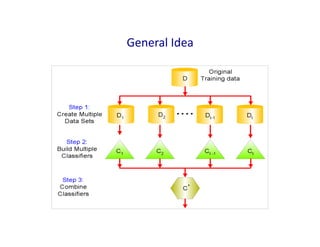
36. Bagging:
Bootstrap
AggregaGon
• Leo
Breiman
(1994)
• Take
repeated
bootstrap
samples
from
training
set
D
• Bootstrap
sampling:
Given
set
D
containing
N
training
examples,
create
D’
by
drawing
N
examples
at
random
with
replacement
from
D.
• Bagging:
– Create
k
bootstrap
samples
D1
…
Dk.
– Train
disGnct
classifier
on
each
Di.
– Classify
new
instance
by
majority
vote
/
average.

37. General
Idea

38. Example
of
Bagging
• Sampling
with
replacement
• Build
classifier
on
each
bootstrap
sample
• Each
data
point
has
probability
(1
–
1/n)n
of
being
selected
as
test
data
• Training
data
=
1-­‐
(1
–
1/n)n
of
the
original
data
Training Data
Data ID

39. 51

40. 52
decision tree learning algorithm; very similar to ID3

41. shades of blue/red indicate strength of vote for particular classification

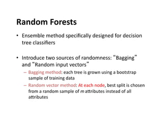
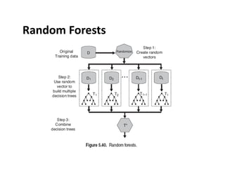
42. Random
Forests
• Ensemble
method
specifically
designed
for
decision
tree
classifiers
• Introduce
two
sources
of
randomness:
“Bagging”
and
“Random
input
vectors”
– Bagging
method:
each
tree
is
grown
using
a
bootstrap
sample
of
training
data
– Random
vector
method:
At
each
node,
best
split
is
chosen
from
a
random
sample
of
m
aIributes
instead
of
all
aIributes

43. Random
Forests

44. Random
Forests
Algorithm