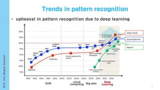
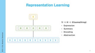
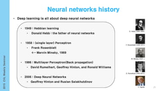
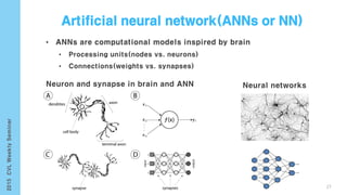
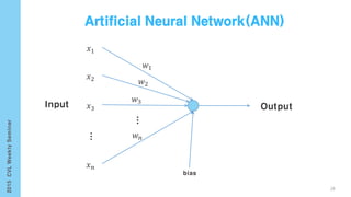
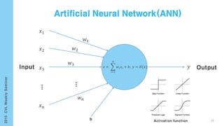
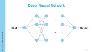
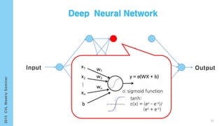
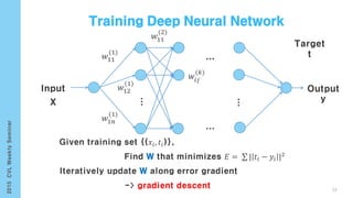
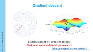
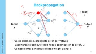
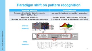
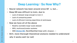
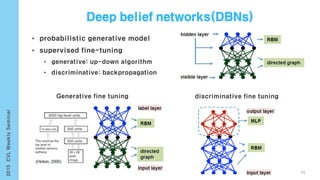
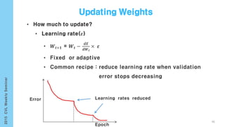
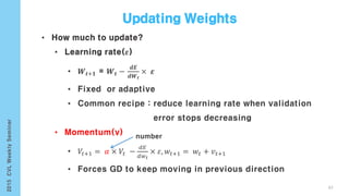
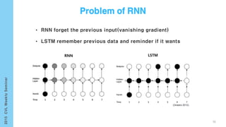
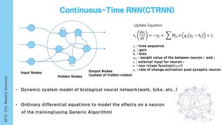
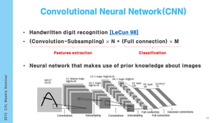
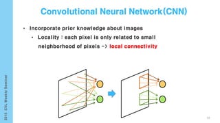
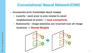
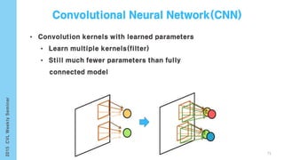
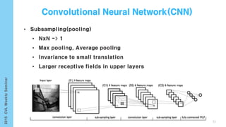
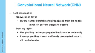
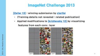
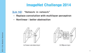
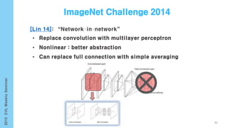
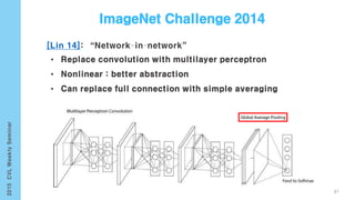
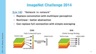
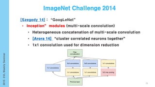
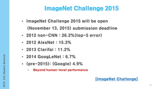
This document provides an overview of the history and development of deep learning and neural networks. It discusses early work in the 1940s-1950s on neural networks and perceptrons. It then covers the development of backpropagation and multi-layer perceptrons in the 1980s which enabled training of deeper models. Recent advances discussed include deep neural networks in 2006 and the shift from shallow to deep learning models around 2006. The document also examines recurrent neural networks, LSTMs, word embeddings, and convolutional neural networks as well as applications in computer vision like image captioning.

1. 1

2. 2

3. 3

4. 4

5. 5

6. 6

7. Car
7

8. Car
HOW?
8

9. H
V
9

10. All
10

11. V
All
H
11

12. All
HV
12

13. All
HV
HVV
13

14. All
HV
HVV
14

15. H VV
V VV
15

16. H VV
V VV
16

17. V V V V V V V V V V
H H H H H
X
17

18. V V V V V V V V V V
H H H H H
X
v v vv v v v
X
18

19. X
h h h h
v v vv v v v
19

20. X
v v vv v v v
h h h h
20

21. X
v v vv v v v
h h h h
21

22. X
v v vv v v v
h h h h
abstraction
abstraction
22

23. X
v v vv v v v
h h h h
abstraction
abstraction
23

24. 24

25. • Deep learning is all about deep neural networks
• 1949 : Hebbian learning
• Donald Hebb : the father of neural networks
• 1958 : (single layer) Perceptron
• Frank Rosenblatt
- Marvin Minsky, 1969
• 1986 : Multilayer Perceptron(Back propagation)
• David Rumelhart, Geoffrey Hinton, and Ronald Williams
• 2006 : Deep Neural Networks
• Geoffrey Hinton and Ruslan Salakhutdinov
25

26. • Weakness in kernel machine(SVM …):
• It does not scale well with sample size.
• Based on matching local templates.
• the training data is referenced for test data
• Local representation VS distributed representation
• N N(Neural Network) -> Kernel machine -> Deep NN
26

27. 27

28. 28

29. 29

30. 30

31. 31

32. 32

33. 33

34. 34

35. 35

36. 36

37. Shallow learning Deep learning
feature extraction by domain experts
(SIFT, SURF, orb...)
automatic feature extraction from data
separate modules
(feature extractor + trainable classifier)
unified model : end-to-end learning
(trainable feature + trainable classifier)
37

38. 38

39. • Core visual object recognition
Feedback
39

40. 40

41. 41

42. 42

43. 43

44. 44

45. 45

46. 46

47. 47

48. 48

49. 49

50. 50

51. 51

52. 52

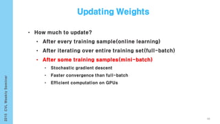
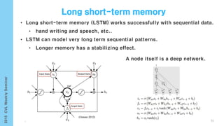
53. 𝑥 𝑡
ℎ 𝑡
=
𝑥0
ℎ0
𝑥2
ℎ2
𝑥1
ℎ1
𝑥 𝑡
ℎ 𝑡
…
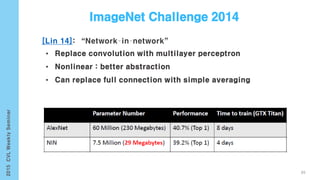
[http://karpathy.github.io/2015/05/21/rnn-effectiveness]53

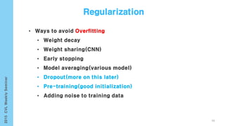
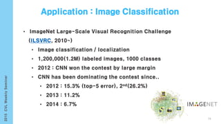
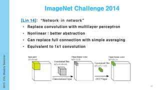
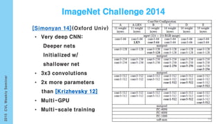
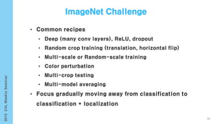
54. • Bidirection Neural Network utilize in the past and future context for
every point in the sequence
• Two Hidden Layer(Forwards and Backwards) shared same output layer
Visualized of the amount of input information for prediction by different network structures
[Schuster 97]
54

55. 55

56. RNN LSTM
• RNN forget the previous input(vanishing gradient)
• LSTM remember previous data and reminder if it wants
56

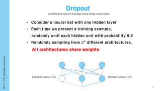
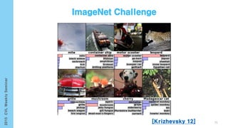
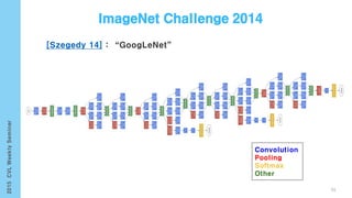
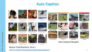
57. ℎ 𝑡−1(𝑝𝑟𝑒𝑣 𝑟𝑒𝑠𝑢𝑙𝑡)
𝜎
𝑥 𝑡(𝑐𝑢𝑟𝑟𝑒𝑛𝑡 𝑑𝑎𝑡𝑎)
𝐶𝑡−1 𝐶𝑡
𝑓𝑡 = 𝜎(𝑊𝑓 ∙ ℎ 𝑡−1, 𝑥 𝑡 + 𝑏𝑓)
𝑓𝑡
[http://colah.github.io/posts/2015-08-Understanding-LSTMs]
57

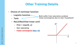
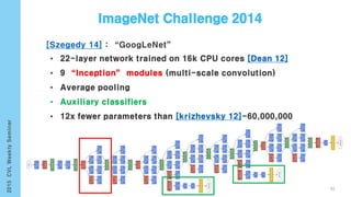
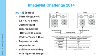
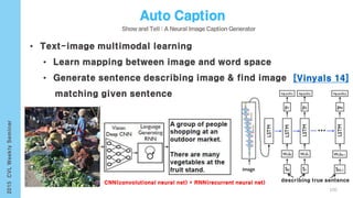
58. ℎ 𝑡−1(𝑝𝑟𝑒𝑣 𝑟𝑒𝑠𝑢𝑙𝑡)
𝜎
𝑥 𝑡(𝑐𝑢𝑟𝑟𝑒𝑛𝑡 𝑑𝑎𝑡𝑎)
𝐶𝑡−1 𝐶𝑡
𝑖 𝑡 = 𝜎(𝑊𝑖 ∙ ℎ 𝑡−1, 𝑥 𝑡 + 𝑏𝑖)
𝜎
𝑓𝑡
𝑖 𝑡
𝑡𝑎𝑛ℎ
𝐶𝑡
𝐶𝑡 = 𝑡𝑎𝑛ℎ(𝑊𝑐 ∙ ℎ 𝑡−1, 𝑥 𝑡 + 𝑏 𝑐)
58
[http://colah.github.io/posts/2015-08-Understanding-LSTMs]

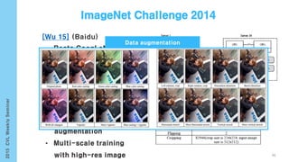
59. ℎ 𝑡−1(𝑝𝑟𝑒𝑣 𝑟𝑒𝑠𝑢𝑙𝑡)
𝜎
𝑥 𝑡(𝑐𝑢𝑟𝑟𝑒𝑛𝑡 𝑑𝑎𝑡𝑎)
𝐶𝑡−1 𝐶𝑡
𝐶𝑡 = 𝑓𝑡 ∗ 𝐶𝑡−1 + 𝑖 𝑡 ∗ 𝐶𝑡
𝜎
𝑓𝑡
𝑖 𝑡
𝑡𝑎𝑛ℎ
𝐶𝑡
ⅹ
+ⅹ
59
[http://colah.github.io/posts/2015-08-Understanding-LSTMs]

60. ℎ 𝑡−1(𝑝𝑟𝑒𝑣 𝑟𝑒𝑠𝑢𝑙𝑡)
𝜎
𝑥 𝑡(𝑐𝑢𝑟𝑟𝑒𝑛𝑡 𝑑𝑎𝑡𝑎)
𝐶𝑡−1 𝐶𝑡
𝑂𝑡 = 𝜎(𝑊𝑜 ∙ ℎ 𝑡−1, 𝑥 𝑡 + 𝑏 𝑜)
𝜎
𝑓𝑡
𝑖 𝑡
𝑡𝑎𝑛ℎ
𝐶𝑡
ⅹ
+ⅹ
𝜎
ⅹ
𝑡𝑎𝑛ℎ
ℎ 𝑡
ℎ 𝑡
ℎ 𝑡 = 𝑂𝑡 ∗ 𝑡𝑎nh(𝐶𝑡)
60
[http://colah.github.io/posts/2015-08-Understanding-LSTMs]

61. 61
• Dropout operator only to non-recurrent connections
[Zaremba14]
Arrow dash applied dropout otherwise solid line is not applied
ℎ 𝑡
𝑙
: hidden state in layer 𝑙 in timestep 𝑡.
dropout operator
Frame-level speech recognition accuracy

62. decode
encode
V1
W1
X2
X1
X1
V1
W1
X2
X1
X1
X2
V2
W2
X3
• Regress from observation to itself (input X1 -> output X1)
• ex : data compression(JPEG etc..)
[Lemme 10]
62
output
hidden
input

63. 0 1 0 0…
0.05 0.7 0.5 0.01…
0.9 0.1 10−8…10−4
cow dog cat bus
original target
output of ensemble
[Hinton 14]
Softened outputs reveal the dark knowledge in the ensemble
dog
dog
training result
cat buscow
dog cat buscow
63

64. • Distribution of the top layer has more information.
• Model size in DNN can increase up to tens of GB
input
target
input
output
Training a DNN
Training a shallow network
64
[Hinton 14]

65. 65
0 1 0 0 0 0 0 0 0 0dog
0 0 1 0 0 0 0 0 0 0cat
• Word embedding 𝑊: 𝑤𝑜𝑟𝑑𝑠 → ℝ 𝑛 function mapping to high-dimensional vectors
0.3 0.2 0.1 0.5 0.7dog
0.2 0.8 0.3 0.1 0.9cat
one hot vector representation
[Vinyals 14]
Nearest neighbors a few words
Word Embedding

66. 𝜏𝑖 : time sequence
𝑔𝑖 : gain
𝑏𝑖 : bias
𝑤𝑗𝑖 : weight value of the between neuron 𝑖 and 𝑗
𝐼𝑖 : external input for neuron 𝑖
𝜎 : non-linear function(𝑡𝑎𝑛ℎ)
𝑦𝑖 : rate of change activation post synaptic neuron
Input Nodes
Hidden Nodes
Output Nodes
(subset of hidden nodes)
𝜏𝑖
𝑑𝑦𝑖
𝑑𝑡
= −𝑦𝑖 + 𝑊𝑗𝑖 𝜎 𝑔𝑗 𝑦𝑗 − 𝑏𝑗 + 𝐼𝑖
Update Equation
66
• Dynamic system model of biological neural network(walk, bike, etc..)
• Ordinary differential equations to model the effects on a neuron
of the training(using Generic Algorithm)

67. 67

68. 68

69. 69

70. 70

71. 71

72. 72

73. 73

74. 74

75. 75

76. 76

77. 77

78. 78

79. 79

80. 80

81. 81

82. 82

83. 83

84. 84

85. 85

86. 86

87. 87

88. 88

89. 89

90. 90

91. 91
Convolution
Pooling
Softmax
Other

92. 92

93. 93

94. 94

95. 95

96. 96
Data augmentation

97. 97
November 13, 2015) submission deadline
• (pre-2015): (Google) 4.9%
• Beyond human-level performance

98. 98

99. 99

100. 100

101. [Karpathy 14]
[Girshick 13]
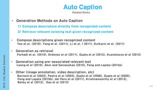
• Generate dense, free-from descriptions of images
Infer region word alignments use to R-CNN + BRNN + MRF
101
Image Segmentation(Graph Cut + Disjoint union)

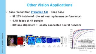
102. [Karpathy 14]
Infer region word alignments use to R-CNN + BRNN + MRF
102
𝑆 𝑘𝑙 =
𝑡∈𝑔 𝑙 𝑖∈𝑔 𝑘
𝑚𝑎𝑥(0, 𝑣𝑖
𝑇
𝑆𝑡)
Result BRNN
Result RNN
𝑔𝑙
𝑔 𝑘
• 𝑆𝑡 and 𝑣𝑖 with their additional
Multiple Instance Learning
hⅹ4096 maxrix(h is 1000~1600)
t-dimensional word dictionary

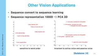
103. [Karpathy 14]
103
𝐸 𝑎1, . . , 𝑎 𝑛 = 𝑎 𝑗=𝑡
−𝑠𝑖𝑚𝑖𝑙𝑎𝑟𝑖𝑡𝑦(𝑤𝑗, 𝑟𝑡) + 𝑗=1..𝑁−1 𝛽[𝑎𝑗 = 𝑎𝑗+1]
Smoothing with an MRF
• Best region independently align each other
• Similarity regions are arrangement nearby
• Argmin can found dynamic programming
(word, region)

104. 104
• Generation Methods on Auto Caption
1) Compose descriptors directly from recognized content
2) Retrieve relevant existing text given recognized content
• Compose descriptions given recognized content
Yao et al. (2010), Yang et al. (2011), Li et al. ( 2011), Kulkarni et al. (2011)
• Generation as retrieval
Farhadi et al. (2010), Ordonez et al (2011), Gupta et al (2012), Kuznetsova et al (2012)
• Generation using pre-associated relevant text
Leong et al (2010), Aker and Gaizauskas (2010), Feng and Lapata (2010a)
• Other (image annotation, video description, etc)
Barnard et al (2003), Pastra et al (2003), Gupta et al (2008), Gupta et al (2009),
Feng and Lapata (2010b), del Pero et al (2011), Krishnamoorthy et al (2012),
Barbu et al (2012), Das et al (2013)

105. 105

106. 106

107. 107

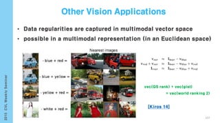
108. • Divided to five part of human body(two arms, two legs, trunk)
• Modeling movements of these individual part and layer composed of 9
layers(BRNN, fusion layer, fully connection layer)
[Yong 15]
108

109. 109

110. 110

111. • “Maching Learning to Deep Learning by 곽동민
• http://www.cs.toronto.edu/~hinton/MatlabForSciencePaper.html
• convolutional neural networks : LeCun
• Alex Krizhevsky: Hinton (python, C++)
• https://code.google.com/p/cuda-convnet/
• Caffe: UC Berkeley (C++)
• http://caffe.berkeleyvision.org/
111

112. 112