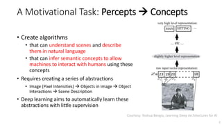
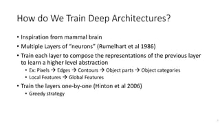
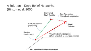
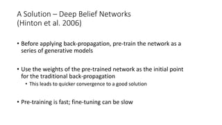
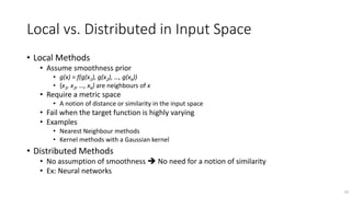
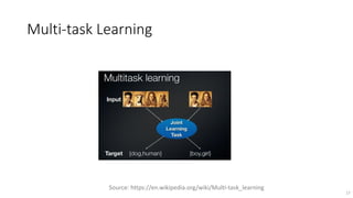
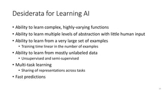
The document provides an introduction to deep learning and discusses some of its key concepts and challenges. It motivates deep learning as a way to create algorithms that can understand scenes and describe them using natural language by automatically learning a series of abstractions from images to concepts. Some challenges discussed include modeling complex behavior with many concepts and interactions. Deep learning approaches like deep belief networks are presented as a way to learn multiple levels of representation from data with little supervision by first pre-training the networks in an unsupervised manner before fine-tuning them for the task.

1. Introduction to Deep Learning
M S Ram
Dept. of Computer Science & Engg.
Indian Institute of Technology Kanpur
Reading of Chap. 1 from “Learning Deep Architectures for AI”; Yoshua Bengio; FTML Vol. 2, No. 1 (2009) 1–127
1
Date: 12 Nov, 2015

2. A Motivational Task: Percepts  Concepts
• Create algorithms
• that can understand scenes and describe
them in natural language
• that can infer semantic concepts to allow
machines to interact with humans using these
concepts
• Requires creating a series of abstractions
• Image (Pixel Intensities)  Objects in Image  Object
Interactions  Scene Description
• Deep learning aims to automatically learn these
abstractions with little supervision
Courtesy: Yoshua Bengio, Learning Deep Architectures for AI
2

3. Deep Visual-Semantic Alignments for Generating
Image Descriptions (Karpathy, Fei-Fei; CVPR 2015)
"boy is doing backflip
on wakeboard."
“two young girls are
playing with lego toy.”
"man in black shirt is
playing guitar."
"construction worker in
orange safety vest is
working on road."
http://cs.stanford.edu/people/karpathy/deepimagesent/
3

4. Challenge in Modelling Complex Behaviour
• Too many concepts to learn
• Too many object categories
• Too many ways of interaction between objects categories
• Behaviour is a highly varying function underlying factors
• f: L  V
• L: latent factors of variation
• low dimensional latent factor space
• V: visible behaviour
• high dimensional observable space
• f: highly non-linear function
4

5. Example: Learning the Configuration Space of a Robotic Arm
5

6. C-Space Discovery using Isomap
6

7. How do We Train Deep Architectures?
• Inspiration from mammal brain
• Multiple Layers of “neurons” (Rumelhart et al 1986)
• Train each layer to compose the representations of the previous layer
to learn a higher level abstraction
• Ex: Pixels  Edges  Contours  Object parts  Object categories
• Local Features  Global Features
• Train the layers one-by-one (Hinton et al 2006)
• Greedy strategy
7

8. Multilayer Perceptron with Back-propagation
First deep learning model (Rumelhart, Hinton, Williams 1986)
input vector
hidden
layers
outputs
Back-propagate
error signal to
get derivatives
for learning
Compare outputs with
correct answer to get
error signal
Source: Hinton’s 2009 tutorial on Deep Belief Networks 8

9. Drawbacks of Back-propagation based Deep Neural
Networks
• They are discriminative models
• Get all the information from the labels
• And the labels don’t give so much of information
• Need a substantial amount of labeled data
• Gradient descent with random initialization leads to poor local
minima

10. Hand-written digit recognition
• Classification of MNIST hand-written digits
• 10 digit classes
• Input image: 28x28 gray scale
• 784 dimensional input

11. A Deeper Look at the Problem
• One hidden layer with 500 neurons
=> 784 * 500 + 500 * 10
≈ 0.4 million weights
• Fitting a model that best explains the training data is an
optimization problem in a 0.4 million dimensional space
• It’s almost impossible for Gradient descent with random
initialization to arrive at the global optimum

12. A Solution – Deep Belief Networks
(Hinton et al. 2006)
Pre-trained
N/W Weights
Fast unsupervised
pre-training
Good
Solution
Slow Fine-tuning
(Using Back-propagation)
Very slow Back-propagation
(Often gets stuck at poor local minima)
Random
Initial position
Very high-dimensional parameter space

13. A Solution – Deep Belief Networks
(Hinton et al. 2006)
• Before applying back-propagation, pre-train the network as a
series of generative models
• Use the weights of the pre-trained network as the initial point
for the traditional back-propagation
• This leads to quicker convergence to a good solution
• Pre-training is fast; fine-tuning can be slow

14. Quick Check: MLP vs DBN on MNIST
• MLP (1 Hidden Layer)
• 1 hour: 2.18%
• 14 hours: 1.65%
• DBN
• 1 hour: 1.65%
• 14 hours: 1.10%
• 21 hours: 0.97%
Intel QuadCore 2.83GHz, 4GB RAM
MLP: Python :: DBN: Matlab

15. Intermediate Representations in Brain
• Disentanglement of factors of variation
underlying the data
• Distributed Representations
• Activation of each neuron is a function of
multiple features of the previous layer
• Feature combinations of different neurons
are not necessarily mutually exclusive
• Sparse Representations
• Only 1-4% neurons are active at a time
15
Localized Representation
Distributed Representation

16. Local vs. Distributed in Input Space
• Local Methods
• Assume smoothness prior
• g(x) = f(g(x1), g(x2), …, g(xk))
• {x1, x2, …, xk} are neighbours of x
• Require a metric space
• A notion of distance or similarity in the input space
• Fail when the target function is highly varying
• Examples
• Nearest Neighbour methods
• Kernel methods with a Gaussian kernel
• Distributed Methods
• No assumption of smoothness  No need for a notion of similarity
• Ex: Neural networks
16

17. Multi-task Learning
17
Source: https://en.wikipedia.org/wiki/Multi-task_learning

18. Desiderata for Learning AI
• Ability to learn complex, highly-varying functions
• Ability to learn multiple levels of abstraction with little human input
• Ability to learn from a very large set of examples
• Training time linear in the number of examples
• Ability to learn from mostly unlabeled data
• Unsupervised and semi-supervised
• Multi-task learning
• Sharing of representations across tasks
• Fast predictions
18

19. References
 Primary
 Yoshua Bengio, Learning Deep Architectures for AI, Foundations and Trends in Machine
Learning Vol. 2, No. 1 (2009) 1–127
 Hinton, G. E., Osindero, S. and Teh, Y. A fast learning algorithm for deep belief nets. Neural
Computation 18 (2006), pp 1527-1554
 Rumelhart, David E., Geoffrey E. Hinton, and R. J. Williams. Learning Internal
Representations by Error Propagation. David E. Rumelhart, James L. McClelland, and the
PDP research group. (editors), Parallel distributed processing: Explorations in the
microstructure of cognition, Volume 1: Foundations. MIT Press, 1986.
 Secondary
 Hinton, G. E., Learning Multiple Layers of Representation, Trends in Cognitive Sciences, Vol.
11, (2007) pp 428-434.
 Hinton G.E., Tutorial on Deep Belief Networks, Machine Learning Summer School,
Cambridge, 2009
 Andrej Karpathy, Li Fei-Fei. Deep Visual-Semantic Alignments for Generating Image
Descriptions. CVPR 2015.