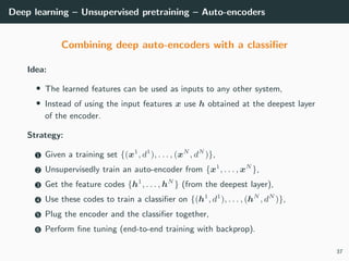
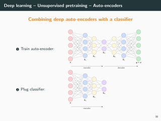
The document outlines the fundamentals of deep learning, including its historical context, key contributors, and applications across various fields like image processing and natural language processing. It details the architecture of artificial neural networks, the principles of representation learning, and the importance of hierarchical feature extraction, as well as challenges such as gradient vanishing and improvements through unsupervised pretraining methods like auto-encoders. Success stories highlight the practical achievements of deep learning, showcasing its transformative impact on technology and machine learning benchmarks.


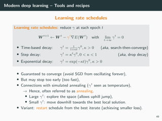


![Modern deep learning – Tools and recipes
Normalized initialization
Idea: A good weight initialization should be random
wij ∼ N(0, σ2
)
Gaussian
or wij ∼ U −
√
3σ,
√
3σ
Uniform
with standard deviation σ chosen such that all (hidden) outputs hj have unit
variance (during the first step of backprop).
Var[hj] = Var g
i
wijhi = 1
Randomness:
prevents units from learning the same thing.
Normalization: preserves dynamic of the
outputs and gradients at each layer:
→ all units get updated with similar speeds.
56](https://image.slidesharecdn.com/3deep-190329010527/85/MLIP-Chapter-3-Introduction-to-deep-learning-65-320.jpg)
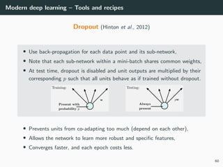
![Modern deep learning – Tools and recipes
Normalized initialization
1 Normalize the inputs with about zero-mean and unit variance,
2 Initialize all the biases to zero,
3 For the weights wij of a unit j with N inputs and activation g:
• Xavier initialization (Glorot & Bengio, 2010): for g(a) = a
Var g
i
wijhi =
i
σ2
Var [hi]
=1
= 1 ⇒ σ =
1
√
N
(Works also for g(a) = tanh(a).)
• He initialization (He et al., 2015): for ReLU → σ =
2
N
(First time, a machine surpasses humans on ImageNet.)
• Kumar initialization (Kumar, 2017): for any g differentiable at 0:
σ2
=
1
Ng (0)2(1 + g(0)2)
57](https://image.slidesharecdn.com/3deep-190329010527/85/MLIP-Chapter-3-Introduction-to-deep-learning-66-320.jpg)


![Attack surfaces and attack tress[inform]](https://cdn.slidesharecdn.com/ss_thumbnails/lecture03-260108015941-a4dee53b-thumbnail.jpg?width=640&height=640&fit=bounds)


