Download as PDF, PPTX


![2.1.
FEED-FORWARD NEURAL NET LANGUAGE MODEL
Bengio et al. (2003)
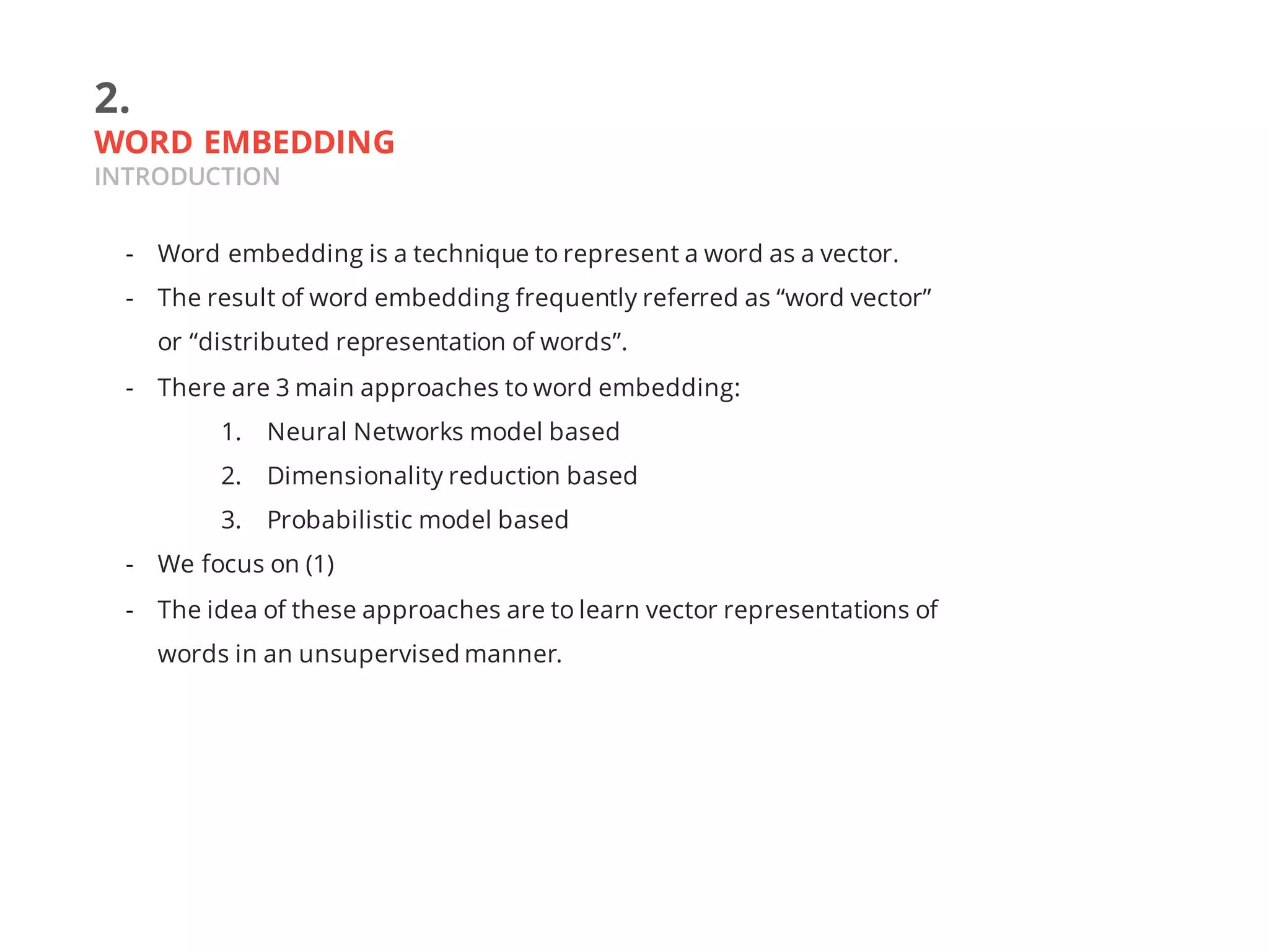
- The training data is a sequence of words 𝑤$, 𝑤& , … , 𝑤] for 𝑤^ ∈ 𝑉
- The model is trying predict the next word 𝑤^ based on the previous
context (previous 𝑛 words: 𝑤^ $,𝑤^ &, … , 𝑤^ a). (Figure 2.1.1)
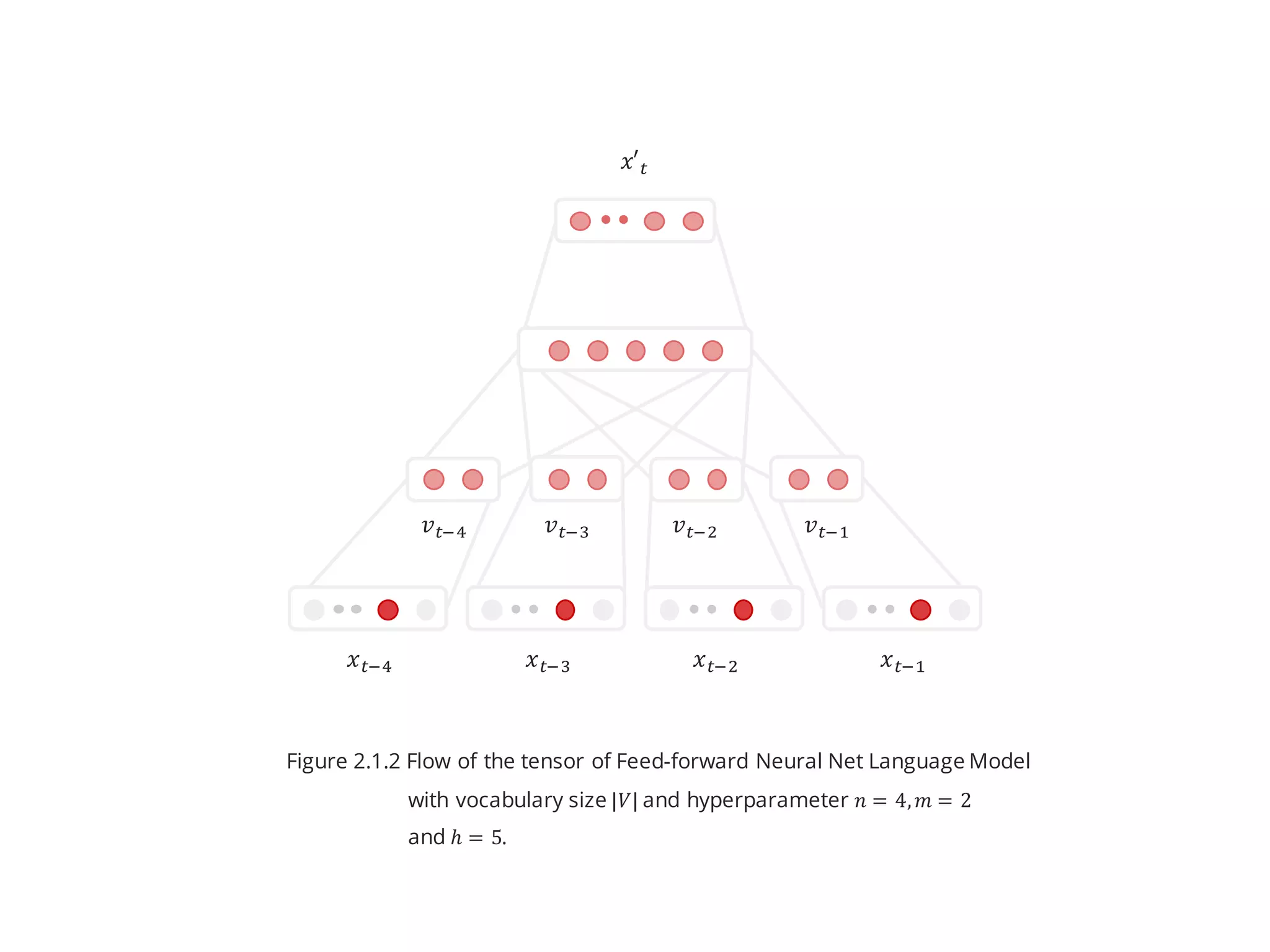
- The model is consist of 4 layers: Input layer, Projection layer, Hidden
layer(s) and output layer. (Figure 2.1.2)
- Known as NNLM
𝑤^
Keren Sale Stock bisa dirumah... ...
𝑤^ $𝑤^ &𝑤^ b𝑤^ c
Figure 2.1.1](https://image.slidesharecdn.com/slidedswjogja2016-clusteringsemanticallysimilarwords-161205101356/75/Clustering-Semantically-Similar-Words-11-2048.jpg)
![2.1.
FEED-FORWARD NEURAL NET LANGUAGE MODEL
COMPOSITION OF FUNCTIONS: INPUT LAYER
- 𝑥^$,𝑥^&,… , 𝑥^a is a 1-of-|𝑉| vector or one-hot-encoded vector of
𝑤^ $, 𝑤^&,… , 𝑤^ a
- 𝑛 is the number of previous words
- The input layer is just acting like placeholder here
𝑥′^ = 𝑓T 𝑥^$,… , 𝑥^a
Output layer : 𝑓T
c
J
= 𝑥′^ = 𝜎 𝑊c]
𝑓T
b
J
+ 𝑏c
Hidden layer : 𝑓T
b
J
= tanh 𝑊b]
𝑓T
&
J
+ 𝑏b
Projection layer : 𝑓T
&
J
= 𝑊&]
𝑓T
$
J
Input layer for i-th example : 𝑓T
$
J = 𝑥^$, 𝑥^&, … , 𝑥^a](https://image.slidesharecdn.com/slidedswjogja2016-clusteringsemanticallysimilarwords-161205101356/75/Clustering-Semantically-Similar-Words-12-2048.jpg)
![2.1.
FEED-FORWARD NEURAL NET LANGUAGE MODEL
COMPOSITION OF FUNCTIONS: PROJECTION LAYER
- The idea of this layer is to project the |𝑉|-dimension vector to
smaller dimension.
- 𝑊&
is the |𝑉|× 𝑚 matrix, also known as embedding matrix, where
each row is a word vector
- Unlike hidden layer, there is no non-linearity here
- This layer also known as “The shared word features layer”
𝑥′^ = 𝑓T 𝑥^$,… , 𝑥^a
Output layer : 𝑓T
c
J
= 𝑥′^ = 𝜎 𝑊c]
𝑓T
b
J
+ 𝑏c
Hidden layer : 𝑓T
b
J
= tanh 𝑊b]
𝑓T
&
J
+ 𝑏b
Projection layer : 𝑓T
&
J
= 𝑊&]
𝑓T
$
J
Input layer for i-th example : 𝑓T
$
J = 𝑥^$, 𝑥^&, … , 𝑥^a](https://image.slidesharecdn.com/slidedswjogja2016-clusteringsemanticallysimilarwords-161205101356/75/Clustering-Semantically-Similar-Words-13-2048.jpg)
![2.1.
FEED-FORWARD NEURAL NET LANGUAGE MODEL
COMPOSITION OF FUNCTIONS: HIDDEN LAYER
- 𝑊b
is the ℎ×𝑛𝑚 matrix where ℎ is the number of hidden units.
- 𝑏b
is a ℎ −dimensional vector.
- The activation function is hyperbolic tangent.
𝑥′^ = 𝑓T 𝑥^$,… , 𝑥^a
Output layer : 𝑓T
c
J
= 𝑥′^ = 𝜎 𝑊c]
𝑓T
b
J
+ 𝑏c
Hidden layer : 𝑓T
b
J
= tanh 𝑊b]
𝑓T
&
J
+ 𝑏b
Projection layer : 𝑓T
&
J
= 𝑊&]
𝑓T
$
J
Input layer for i-th example : 𝑓T
$
J = 𝑥^$, 𝑥^&, … , 𝑥^a](https://image.slidesharecdn.com/slidedswjogja2016-clusteringsemanticallysimilarwords-161205101356/75/Clustering-Semantically-Similar-Words-14-2048.jpg)
![2.1.
FEED-FORWARD NEURAL NET LANGUAGE MODEL
COMPOSITION OF FUNCTIONS: OUPTUT LAYER
- 𝑊c
is the ℎ×|𝑉| matrix.
- 𝑏c
is a |𝑉|-dimensional vector.
- The activation function is softmax.
- 𝑥′^ is a |𝑉|-dimensional vector.
𝑥′^ = 𝑓T 𝑥^$,… , 𝑥^a
Output layer : 𝑓T
c
J
= 𝑥′^ = 𝜎 𝑊c]
𝑓T
b
J
+ 𝑏c
Hidden layer : 𝑓T
b
J
= tanh 𝑊b]
𝑓T
&
J
+ 𝑏b
Projection layer : 𝑓T
&
J
= 𝑊&]
𝑓T
$
J
Input layer for i-th example : 𝑓T
$
J = 𝑥^$, 𝑥^&, … , 𝑥^a](https://image.slidesharecdn.com/slidedswjogja2016-clusteringsemanticallysimilarwords-161205101356/75/Clustering-Semantically-Similar-Words-15-2048.jpg)
![2.2.
CONTINUOUS BAG-OF-WORDS MODEL
Mikolov et al. (2013)
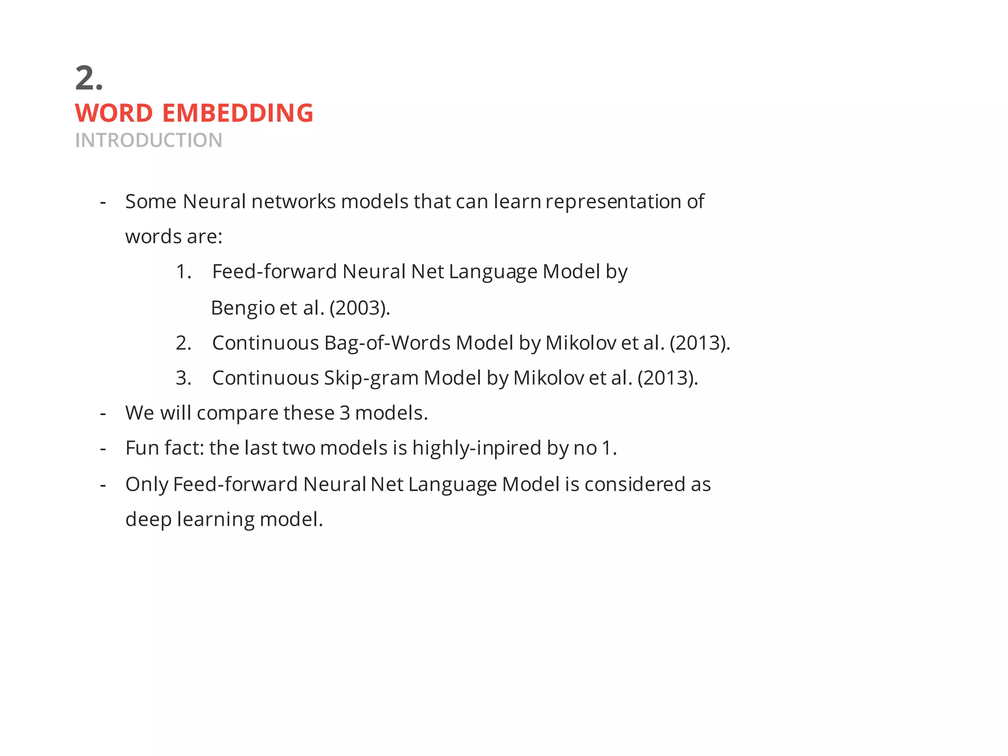
- The training data is a sequence of words 𝑤$, 𝑤& , … , 𝑤] for 𝑤^ ∈ 𝑉
- The model is trying predict the word 𝑤^ based on the surrounding
context (𝑛 words from left: 𝑤^$,𝑤^ & and 𝑛 words from the right:
𝑤^ $, 𝑤^&). (Figure 2.2.1)
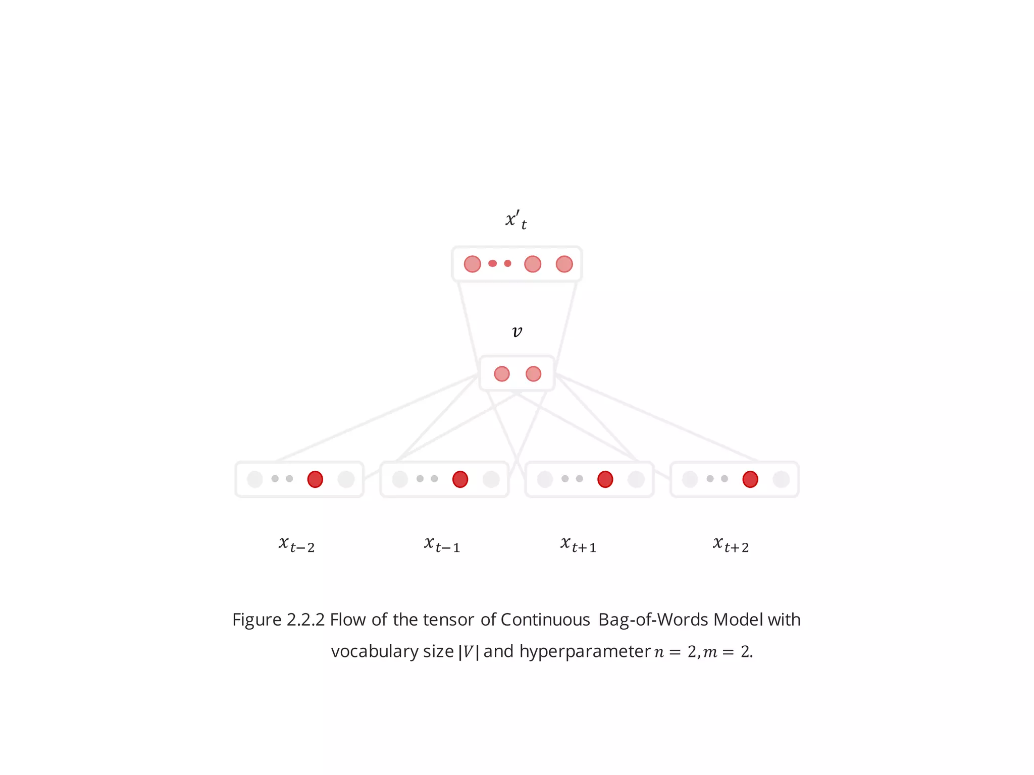
- There are no hidden layer in this model.
- Projection layer is averaged across input words.
𝑤^ x&
Keren Sale bisa bayar dirumah... ...
𝑤^ x$𝑤^𝑤^ $𝑤^ &
Figure 2.2.1](https://image.slidesharecdn.com/slidedswjogja2016-clusteringsemanticallysimilarwords-161205101356/75/Clustering-Semantically-Similar-Words-18-2048.jpg)
![2.2.
CONTINUOUS BAG-OF-WORDS MODEL
COMPOSITION OF FUNCTIONS: INPUT LAYER
- 𝑥^y is a 1-of-|𝑉| vector or one-hot-encoded vector of 𝑤^y.
- 𝑛 is the number of words on the left and the right.
𝑥′^ = 𝑓T 𝑥^a, … , 𝑥^$,𝑥^x$, …, 𝑥^xa
Output layer : 𝑓T
b
J
= 𝑥′^ = 𝜎 𝑊b]
𝑓T
&
J
+ 𝑏b
Projection layer : 𝑓T
&
J
= 𝑣 =
1
2𝑛
n 𝑊&]
𝑓T
$
(𝑗) J
a{y{a,y|}
y
Input layer for i-th example : 𝑓T
$
(𝑗) J = 𝑥^y, −𝑛 ≤ 𝑗 ≤ 𝑛, 𝑗 ≠ 0](https://image.slidesharecdn.com/slidedswjogja2016-clusteringsemanticallysimilarwords-161205101356/75/Clustering-Semantically-Similar-Words-19-2048.jpg)
![2.2.
CONTINUOUS BAG-OF-WORDS MODEL
COMPOSITION OF FUNCTIONS: PROJECTION LAYER
- The difference from previous model is this model project all the
inputs to one 𝑚-dimensional vector 𝑣.
- 𝑊&
is the |𝑉|× 𝑚 matrix, also known as embedding matrix, where
each row is a word vector.
𝑥′^ = 𝑓T 𝑥^a, … , 𝑥^$,𝑥^x$, …, 𝑥^xa
Output layer : 𝑓T
b
J
= 𝑥′^ = 𝜎 𝑊b]
𝑓T
&
J
+ 𝑏b
Projection layer : 𝑓T
&
J
= 𝑣 =
1
2𝑛
n 𝑊&]
𝑓T
$
(𝑗) J
a{y{a,y|}
y
Input layer for i-th example : 𝑓T
$
(𝑗) J = 𝑥^y, −𝑛 ≤ 𝑗 ≤ 𝑛, 𝑗 ≠ 0](https://image.slidesharecdn.com/slidedswjogja2016-clusteringsemanticallysimilarwords-161205101356/75/Clustering-Semantically-Similar-Words-20-2048.jpg)
![2.2.
CONTINUOUS BAG-OF-WORDS MODEL
COMPOSITION OF FUNCTIONS: OUPTUT LAYER
- 𝑊b
is the m×|𝑉| matrix.
- 𝑏b
is a |𝑉|-dimensional vector.
- The activation function is softmax.
- 𝑥′^ is a |𝑉|-dimensional vector.
𝑥′^ = 𝑓T 𝑥^a, … , 𝑥^$,𝑥^x$, …, 𝑥^xa
Output layer : 𝑓T
b
J
= 𝑥′^ = 𝜎 𝑊b]
𝑓T
&
J
+ 𝑏b
Projection layer : 𝑓T
&
J
= 𝑣 =
1
2𝑛
n 𝑊&]
𝑓T
$
(𝑗) J
a{y{a,y|}
y
Input layer for i-th example : 𝑓T
$
(𝑗) J = 𝑥^y, −𝑛 ≤ 𝑗 ≤ 𝑛, 𝑗 ≠ 0](https://image.slidesharecdn.com/slidedswjogja2016-clusteringsemanticallysimilarwords-161205101356/75/Clustering-Semantically-Similar-Words-21-2048.jpg)
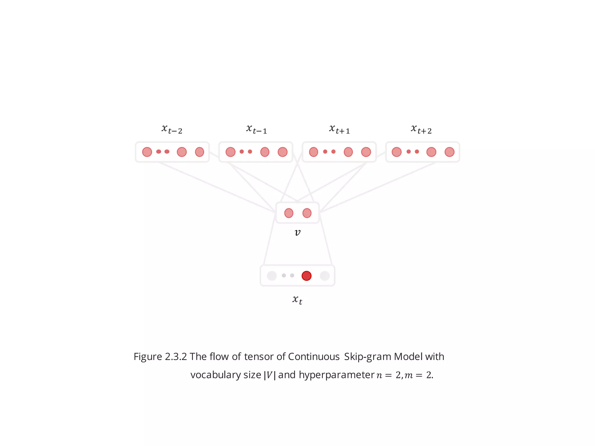
![2.3.
CONTINUOUS SKIP-GRAM MODEL
Mikolov et al. (2013)
- The training data is a sequence of words 𝑤$, 𝑤& , … , 𝑤] for 𝑤^ ∈ 𝑉
- The model is trying predict the surrounding context (𝑛 words from
left: 𝑤^$,𝑤^ & and 𝑛 words from the right: 𝑤^ $,𝑤^ &) based on the
word 𝑤^ . (Figure 2.3.1)
𝑤^ x&
Keren bisa... ...
𝑤^ x$𝑤^𝑤^ $𝑤^ &
Figure 2.3.1](https://image.slidesharecdn.com/slidedswjogja2016-clusteringsemanticallysimilarwords-161205101356/75/Clustering-Semantically-Similar-Words-24-2048.jpg)
![2.3.
CONTINUOUS SKIP-GRAM MODEL
COMPOSITION OF FUNCTIONS: INPUT LAYER
- 𝑥^ is a 1-of-|𝑉| vector or one-hot-encoded vector of 𝑤^ .
𝑋′ = 𝑓T 𝑥^
Output layer : 𝑓T
b
J
= 𝑋′ = 𝜎 𝑊b]
𝑓T
&
J
+ 𝑏b
Projection layer : 𝑓T
&
J
= 𝑊&]
𝑓T
$
J
Input layer for i-th example : 𝑓T
$
J = 𝑥^](https://image.slidesharecdn.com/slidedswjogja2016-clusteringsemanticallysimilarwords-161205101356/75/Clustering-Semantically-Similar-Words-25-2048.jpg)
![2.3.
CONTINUOUS SKIP-GRAM MODEL
COMPOSITION OF FUNCTIONS: PROJECTION LAYER
- 𝑊&
is the |𝑉|× 𝑚 matrix, also known as embedding matrix, where
each row is a word vector.
- Same as Continuous Bag-of-Words model
𝑋′ = 𝑓T 𝑥^
Output layer : 𝑓T
b
J
= 𝑋′ = 𝜎 𝑊b]
𝑓T
&
J
+ 𝑏b
Projection layer : 𝑓T
&
J
= 𝑊&]
𝑓T
$
J
Input layer for i-th example : 𝑓T
$
J = 𝑥^](https://image.slidesharecdn.com/slidedswjogja2016-clusteringsemanticallysimilarwords-161205101356/75/Clustering-Semantically-Similar-Words-26-2048.jpg)
![2.3.
CONTINUOUS SKIP-GRAM MODEL
COMPOSITION OF FUNCTIONS: OUTPUT LAYER
- 𝑊b
is the m×2𝑛|𝑉| matrix.
- 𝑏b
is a 2n|𝑉|-dimensional vector.
- The activation function is softmax.
- 𝑋‚
is a 2n|𝑉|-dimensional vector can be written as
𝑋′ = 𝑓T 𝑥^
Output layer : 𝑓T
b
J
= 𝑋′ = 𝜎 𝑊b]
𝑓T
&
J
+ 𝑏b
Projection layer : 𝑓T
&
J
= 𝑊&]
𝑓T
$
J
Input layer for i-th example : 𝑓T
$
J = 𝑥^
𝑋‚
= (𝑝(𝑤^a |𝑤^ ), … , 𝑝(𝑤^$ |𝑤^ ), 𝑝(𝑤^x$|𝑤^ ),… , 𝑝(𝑤^xa |𝑤^ ))](https://image.slidesharecdn.com/slidedswjogja2016-clusteringsemanticallysimilarwords-161205101356/75/Clustering-Semantically-Similar-Words-27-2048.jpg)


The document provides a detailed overview of clustering semantically similar words using deep learning models in natural language processing. It covers techniques such as word embedding, different neural network models for word representation, similarity metrics, and consensus clustering algorithms. The document also includes a case study and resources for further exploration.


![[DSC Europe 25] Kaja Kandare - LLM as a judge.pptx](https://cdn.slidesharecdn.com/ss_thumbnails/arxyccaxsdsd1ba99wjw-7-251212104007-2b4e3f64-thumbnail.jpg?width=640&height=640&fit=bounds)


![[DSC Europe 25] Branko Dzakula - From Defense to Attack: How AI Redefines Cyb...](https://cdn.slidesharecdn.com/ss_thumbnails/80bdzdxpr3ky2g0qvyk9-8-251211083048-ce5fc1ee-thumbnail.jpg?width=640&height=640&fit=bounds)
![[DSC Europe 25] Branko Urosevic -Rethinking Financial Talent: Integrating Cod...](https://cdn.slidesharecdn.com/ss_thumbnails/8jjrus8ttko6qj64f58f-3-251212103250-642c6374-thumbnail.jpg?width=640&height=640&fit=bounds)


![[DSC Europe 25] Bassam Maharmeh - Artificial Intelligence: Opportunities and ...](https://cdn.slidesharecdn.com/ss_thumbnails/thhfmr2fqpawzj7hsjpg-5-251211083048-2c23204f-thumbnail.jpg?width=640&height=640&fit=bounds)


![[DSC Europe 25] Uros Pesic - The Reality of AI in Marketing.pdf](https://cdn.slidesharecdn.com/ss_thumbnails/rtkodnmtycovsllvzsyn-9-251215095918-b0c6bfe3-thumbnail.jpg?width=640&height=640&fit=bounds)
![[DSC Europe 25] Debmalya Biswas - Agentification: the art of transforming man...](https://cdn.slidesharecdn.com/ss_thumbnails/r5azlggvtqiaiiusrqdr-4-251212103249-5a12c89b-thumbnail.jpg?width=640&height=640&fit=bounds)

![[DSC Europe 25] Tatevik Maytesyan - How to actually use AI in marketing: gett...](https://cdn.slidesharecdn.com/ss_thumbnails/tjo626lsqdgfntbgl2mw-4-251216103155-e36cd239-thumbnail.jpg?width=640&height=640&fit=bounds)


![[DSC Europe 25] Danica Soc - The Science Behind Marketing: Experimentation me...](https://cdn.slidesharecdn.com/ss_thumbnails/c0nofsggs9gw5ucmallr-3-251216103155-56bd64d1-thumbnail.jpg?width=640&height=640&fit=bounds)