Download to read offline


![11
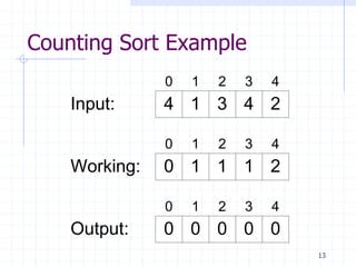
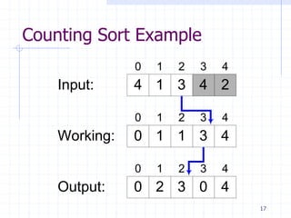
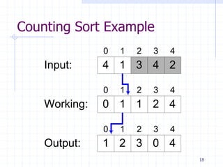
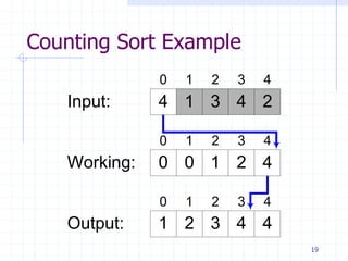
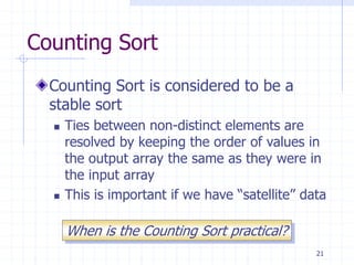
Counting Sort
void CountingSort(int Input[], int Output[], int size,
int max)
{
int Work[max] = { 0 }, index;
// Set Work[i] equal to the # elements = i
for ( index = 0 ; index < size ; ++ index )
Work[Input[index]] = Work[Input[index]] + 1;
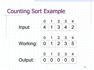
// Now set each Work[i] equal to # elements <= i
for ( index = 2 ; index < max ; ++ index )
Work[index] = Work[index]+Work[index-1];
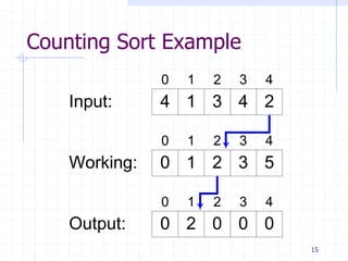
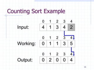
// Arrange the input into the output array
for ( index = size-1 ; index >= 0 ; --index )
{
--Work[Input[index]]; // Handles non-distinct input
Output[Work[Input[index]]] = Input[index];
}
}](https://image.slidesharecdn.com/cis435week06-140325165939-phpapp01/85/Cis435-week06-11-320.jpg)
![27
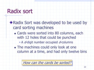
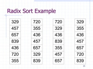
Radix Sort Algorithm
void RadixSort(ArrayType Input[], int size, int digits)
{
for ( int i = 0 ; i < digits ; ++i )
// perform stable sort on Input using digit i
}](https://image.slidesharecdn.com/cis435week06-140325165939-phpapp01/85/Cis435-week06-27-320.jpg)
![31
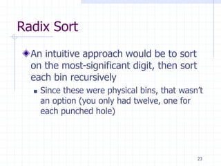
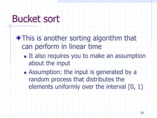
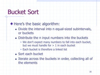
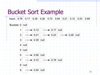
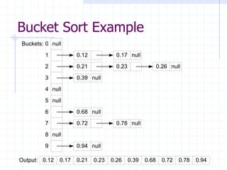
Bucket Sort Algorithm
void BucketSort(double Input[], int size)
{
list<double> buckets[size];
for ( int idx = 0 ; idx < size ; ++idx )
buckets[n*Input[idx]].insert(Input[idx]);
for ( int idx = 0 ; idx < size ; ++idx )
insertion_sort(buckets[idx]);
// concatenate all buckets
}](https://image.slidesharecdn.com/cis435week06-140325165939-phpapp01/85/Cis435-week06-31-320.jpg)


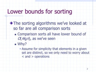
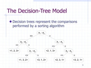
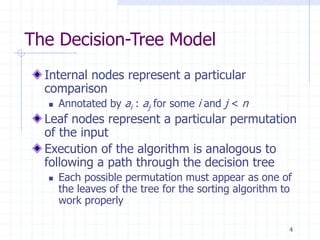
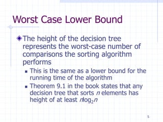
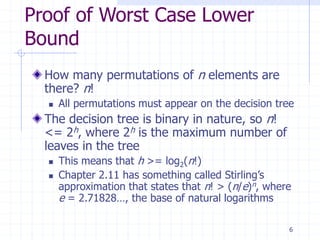
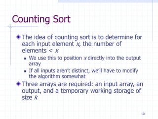
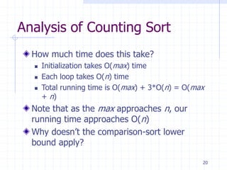
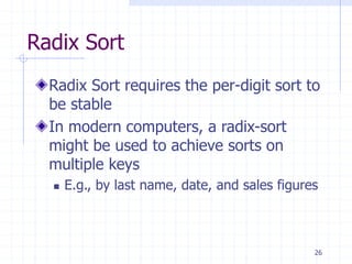
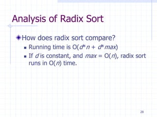
1. Counting sort and radix sort can sort in linear time O(n) by exploiting properties of the input rather than just comparisons. Counting sort assumes integers as input and radix sort assumes digitized numbers. 2. Bucket sort also runs in linear time if inputs are uniformly distributed between 0 and 1. It divides the range into buckets and distributes inputs into the corresponding buckets which are then sorted. 3. The comparison-based lower bound of Ω(nlogn) does not apply to these algorithms because they do not rely solely on comparisons. Counting sort counts occurrences rather than comparing, and radix/bucket sort distribute into buckets based on digits/positions rather than comparisons.