Downloaded 15 times


![Sorting Methods Based on D&C
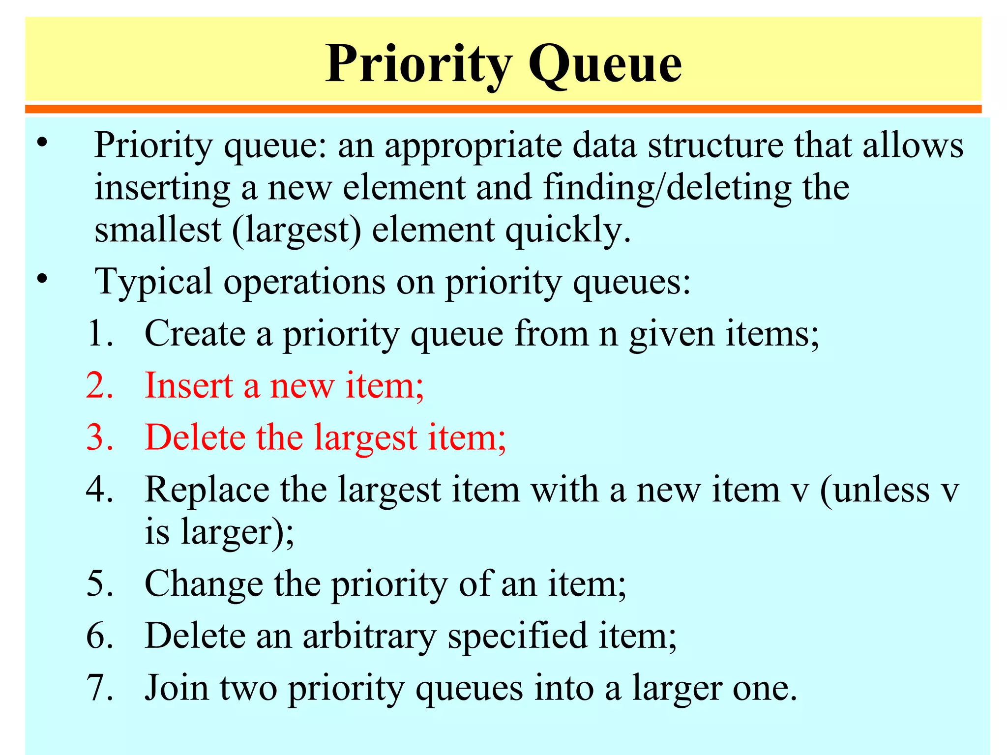
• Big Question: How to divide input file?
• Divide based on number of elements (and not their
values):
– Divide into files of size 1 and n-1
• Insertion sort
–Sort A[1], ..., A[n-1]
–Insert A[n] into proper place.
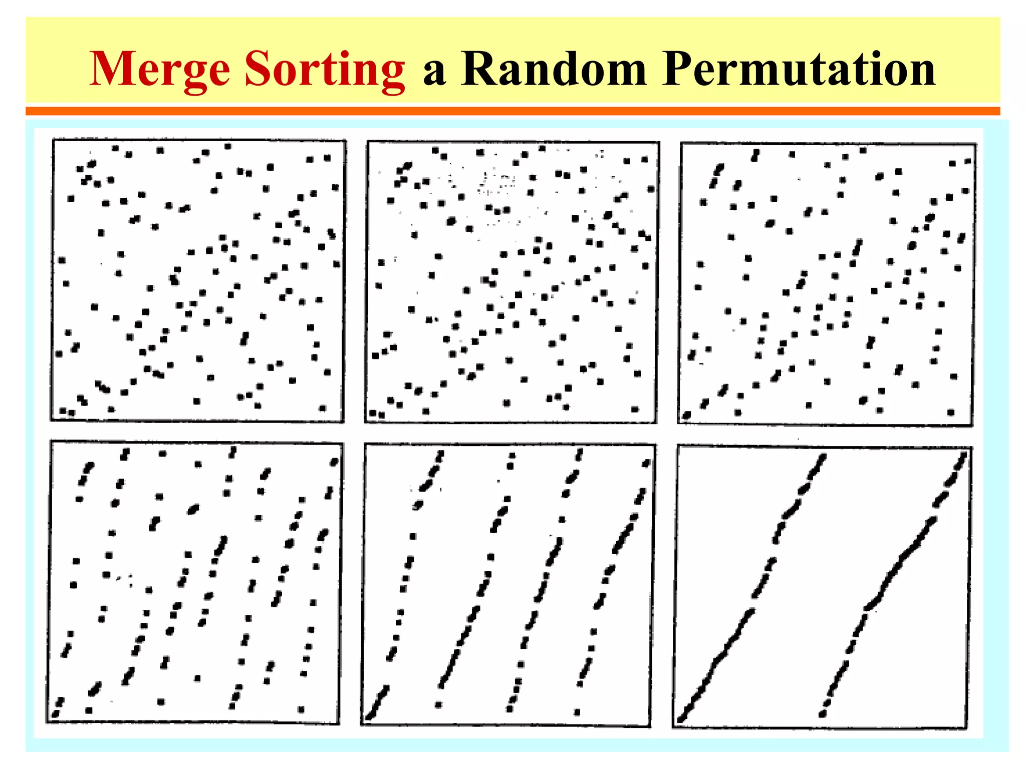
– Divide into files of size n/2 and n/2
• Mergesort
–Sort A[1], ..., A[n/2]
–Sort A[n/2+1], ..., A[n]
–Merge together.
– For these methods, divide is trivial, merge is](https://image.slidesharecdn.com/a13-sorting-150613071621-lva1-app6892/75/sorting-7-2048.jpg)
![Sorting Methods Based on D&C
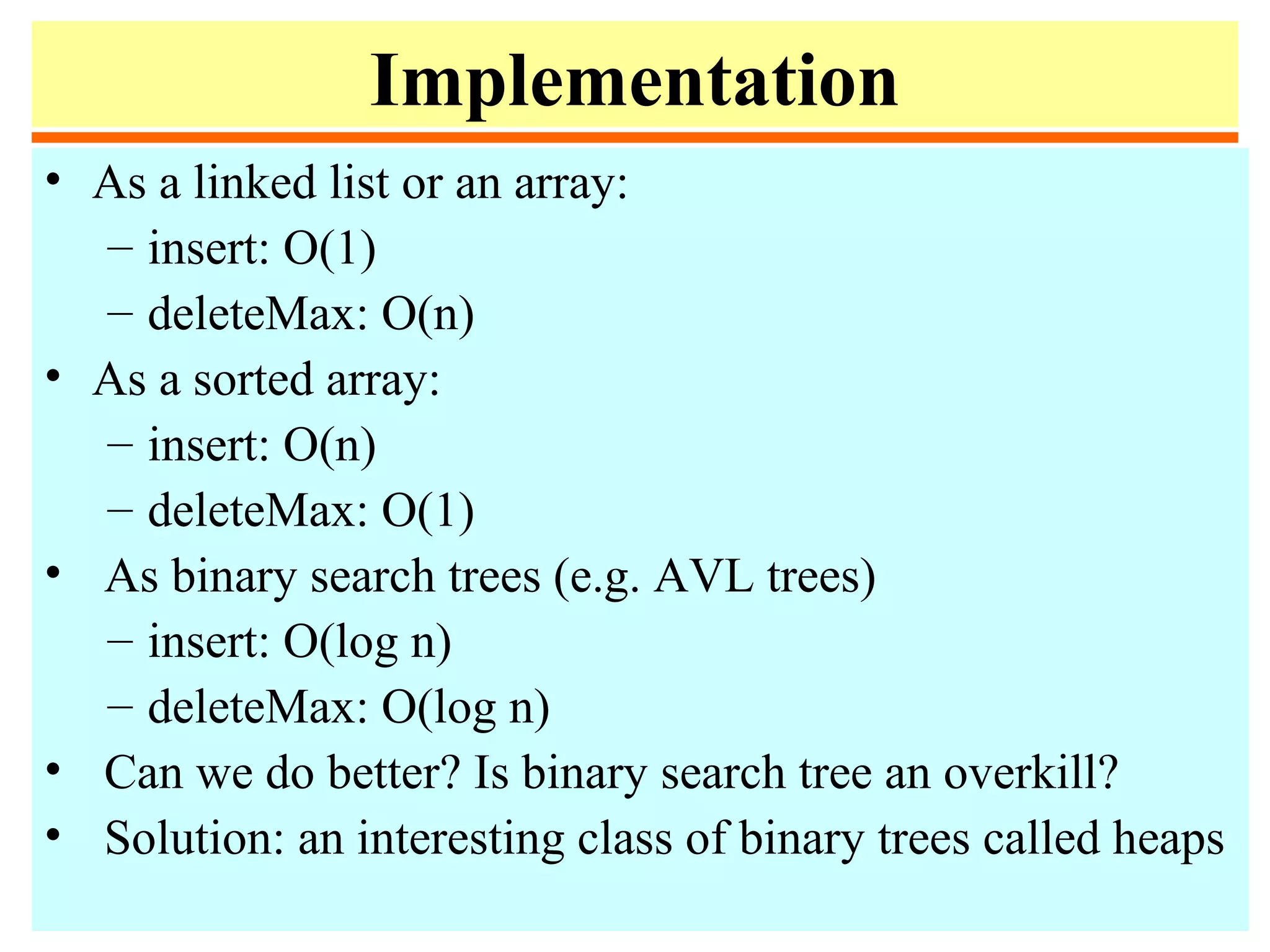
• Divide file based on some values:
– Divide based on the minimum (or maximum)
• Selection sort, Bubble sort, Heapsort
–Find the minimum of the file
–Move it to position 1
–Sort A[2], ..., A[n].
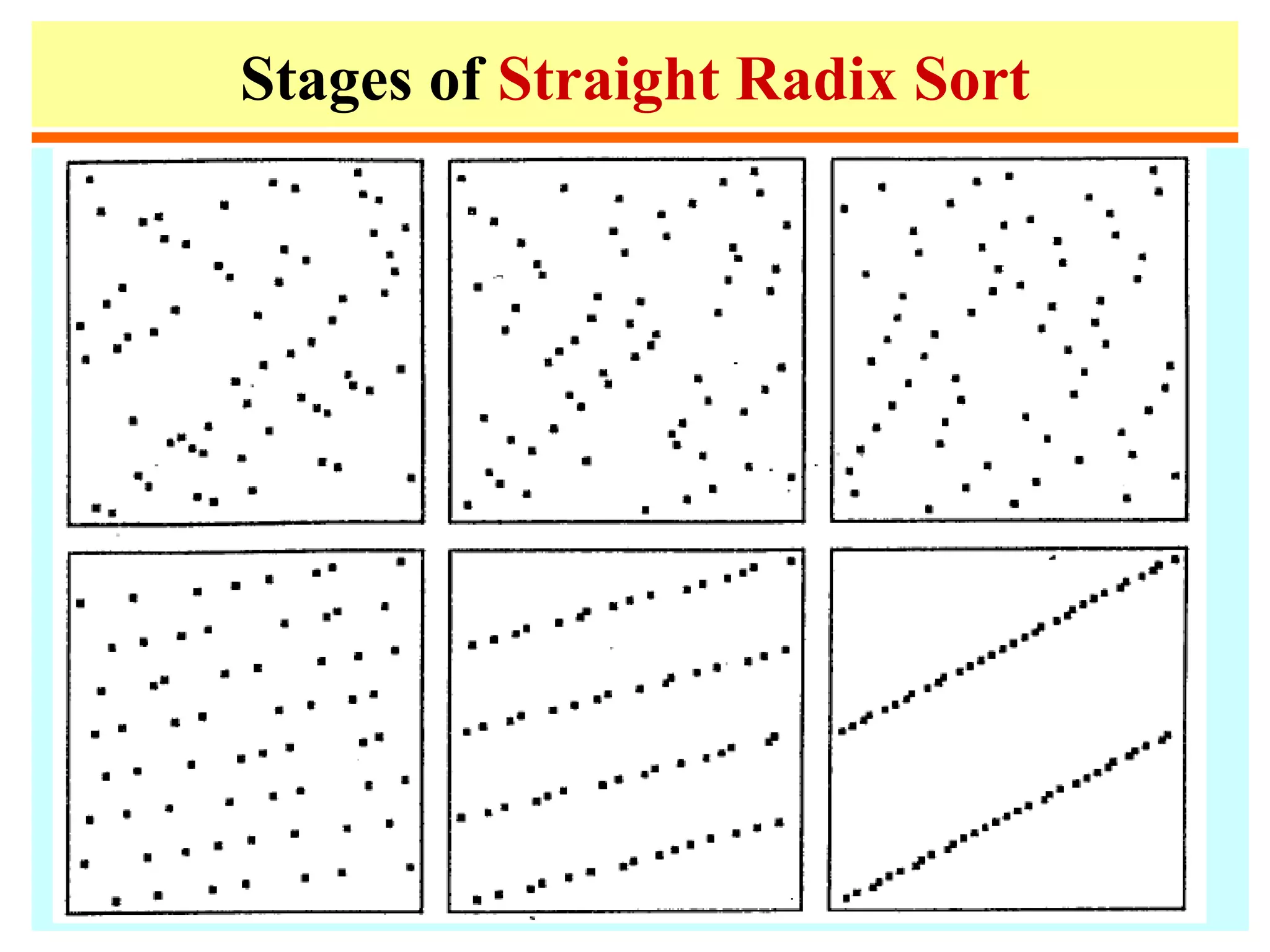
– Divide based on some value (Radix sort, Quicksort)
• Quicksort
–Partition the file into 3 subfiles consisting of:
elements < A[1], = A[1], and > A[1]
–Sort the first and last subfiles
–Form total file by concatenating the 3 subfiles.
– For these methods, divide is non-trivial, merge is
trivial.](https://image.slidesharecdn.com/a13-sorting-150613071621-lva1-app6892/75/sorting-8-2048.jpg)
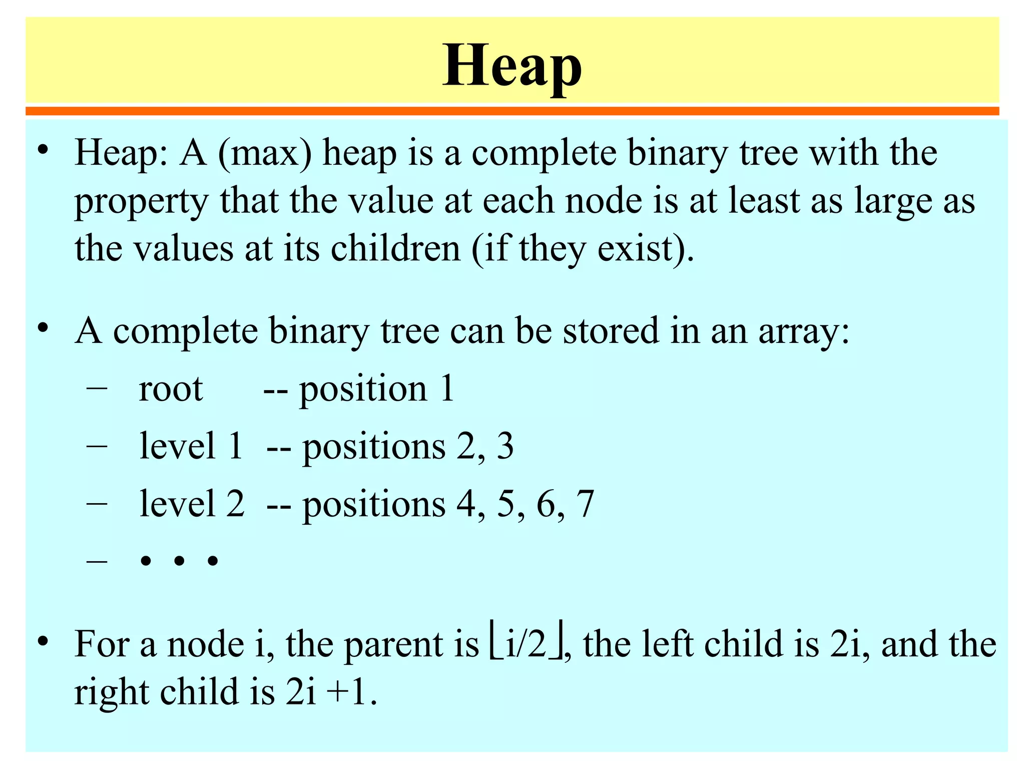
![Selection Sort
3 6 2 7 4 8 11 5
1 6 22 7 4 8 3 5
1 2 6 7 4 8 33 5
1 2 3 7 44 8 6 5
1 2 3 4 7 8 6 55
1 2 3 4 5 8 66 7
1 2 3 4 5 6 8 77
1 2 3 4 5 6 7 8
n exchanges
n2
/2 comparisons
1. for i := 1 to n-1 do
2. begin
3. min := i;
4. for j := i + 1 to n do
5. if a[j] < a[min] then min := j;
6. swap(a[min], a[i]);
7. end;
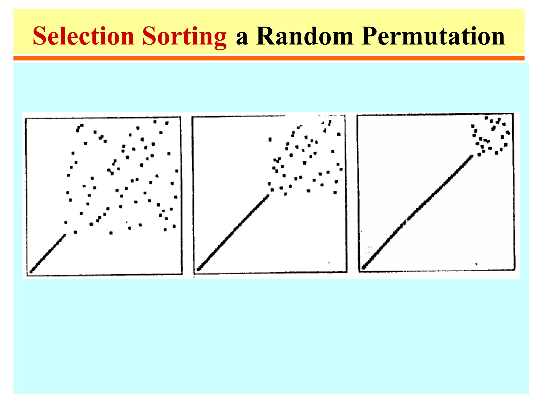
• Selection sort is linear for files with large
record and small keys](https://image.slidesharecdn.com/a13-sorting-150613071621-lva1-app6892/75/sorting-9-2048.jpg)
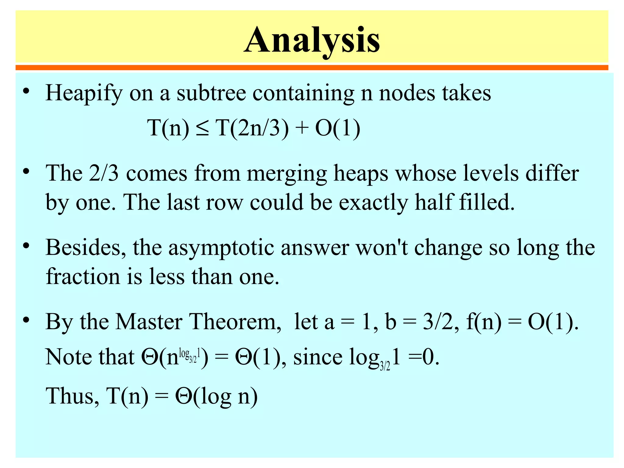
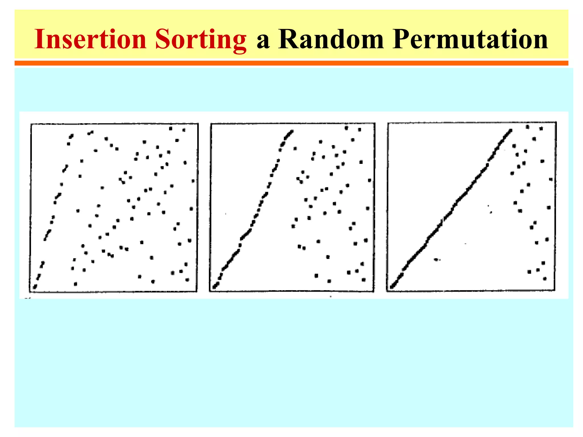
![Insertion Sort
3 6 22 7 4 8 1 5
2 3 6 7 44 8 1 5
2 3 4 6 7 8 11 5
1 2 3 4 6 7 8 55
1 2 3 4 5 6 7 8
n2
/4 exchanges
n2
/4 comparisons
1. for i := 2 to n do
2. begin
3. v := a[i]; j := i;
4. while a[j-1] > v do
5. begin a[j] := a[j-1]; j := j-1 end;
6. a[j] := v;
7. end;
• linear for "almost sorted" files
• Binary insertion sort: Reduces
comparisons but not moves.
• List insertion sort: Use linked list,
no moves, but must use sequential
search.](https://image.slidesharecdn.com/a13-sorting-150613071621-lva1-app6892/75/sorting-10-2048.jpg)
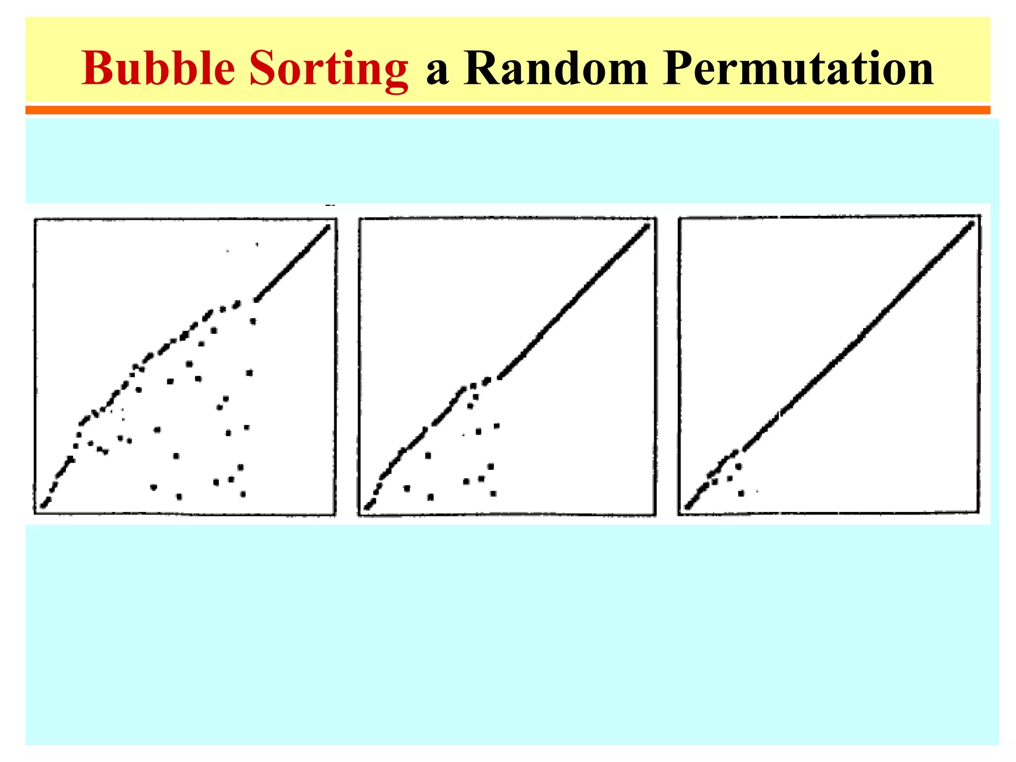
![Bubble Sort
3 6 2 7 4 8 11 5
3 2 6 4 7 11 5 8
2 3 4 6 11 5 7 8
2 3 4 11 5 6 7 8
2 3 11 4 5 6 7 8
2 11 3 4 5 6 7 8
11 2 3 4 5 6 7 8
1. for i := n down to 1 do
2. for j := 2 to i do
3. if a[j-1] > a[j]
then swap(a[j], a[j-1]);
• n2
/4 exchanges
• n2
/2 comparisons
• Bubble can be improved by
adding a flag to check if the list
has already been sorted.](https://image.slidesharecdn.com/a13-sorting-150613071621-lva1-app6892/75/sorting-11-2048.jpg)
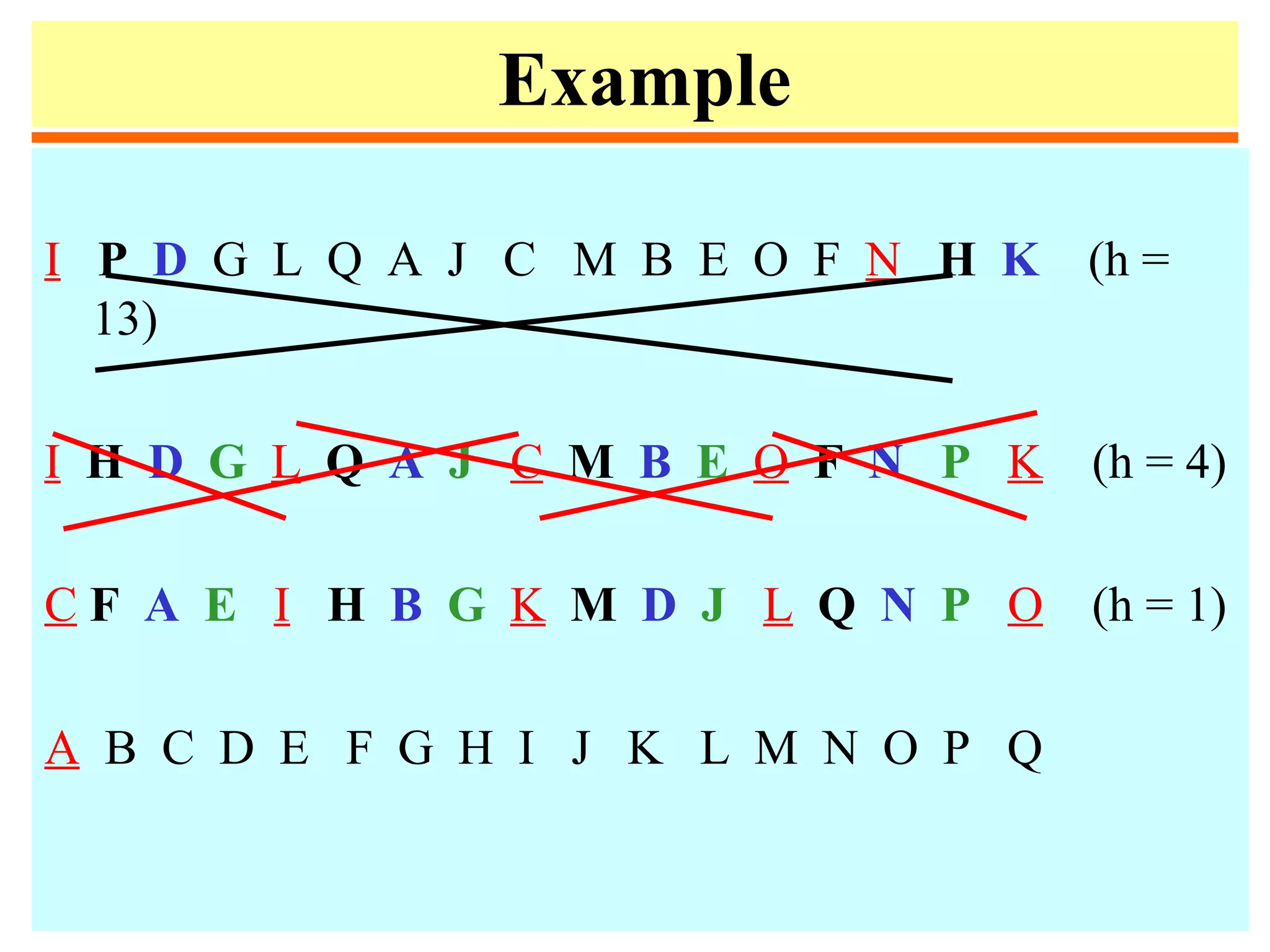
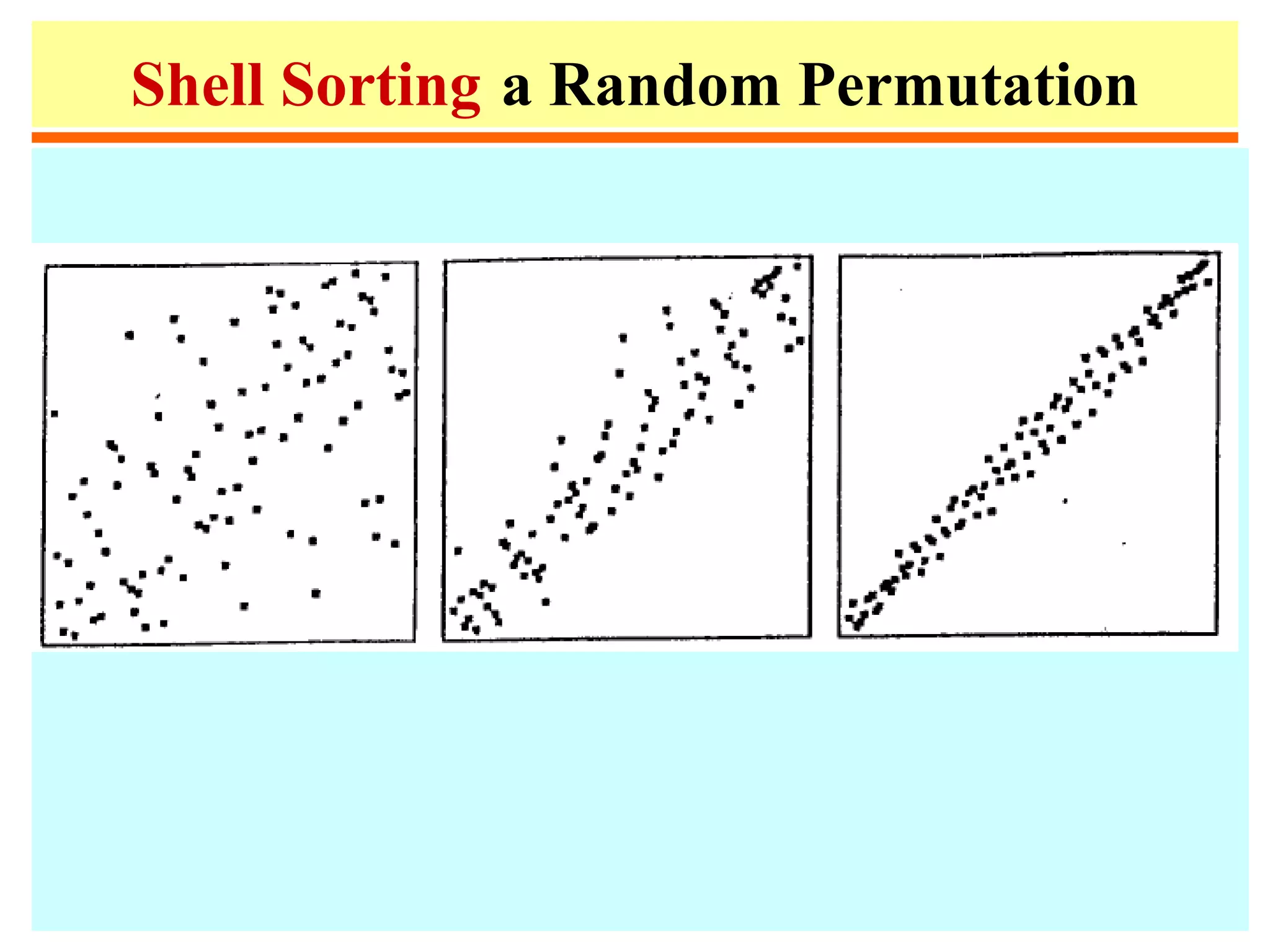
![Shell Sort
h := 1;
repeat h := 3*h+1 until
h>n;
repeat
h := h div 3;
for i := h+1 to n do
begin
v := a[i]; j:= i;
while j>h & a[j-h]>v do
begin
a[j] := a[j-h]; j := j -
h;
end;
a[j] := v;
• Shellsort is a simple extension of
insertion sort, which gains
speeds by allowing exchange of
elements that are far apart.
• Idea: rearrange list into h-sorted
(for any sequence of values of h
that ends in 1.)
• Shellsort never does more than
n1.5
comparisons (for the h = 1, 4,
13, 40, ...).
• The analysis of this algorithm is
hard. Two conjectures of the
complexity are n(log n)2
and n1.25](https://image.slidesharecdn.com/a13-sorting-150613071621-lva1-app6892/75/sorting-12-2048.jpg)
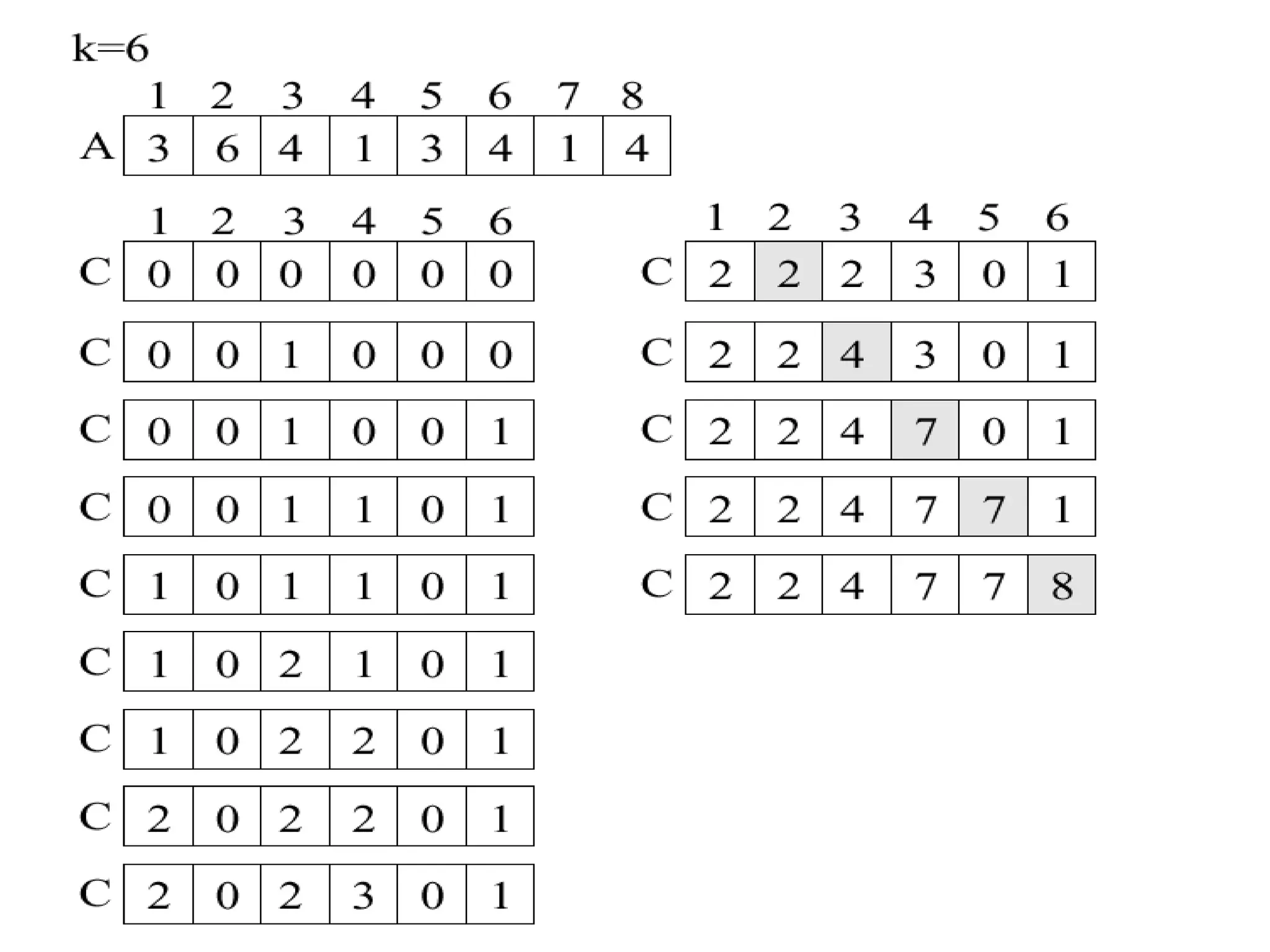
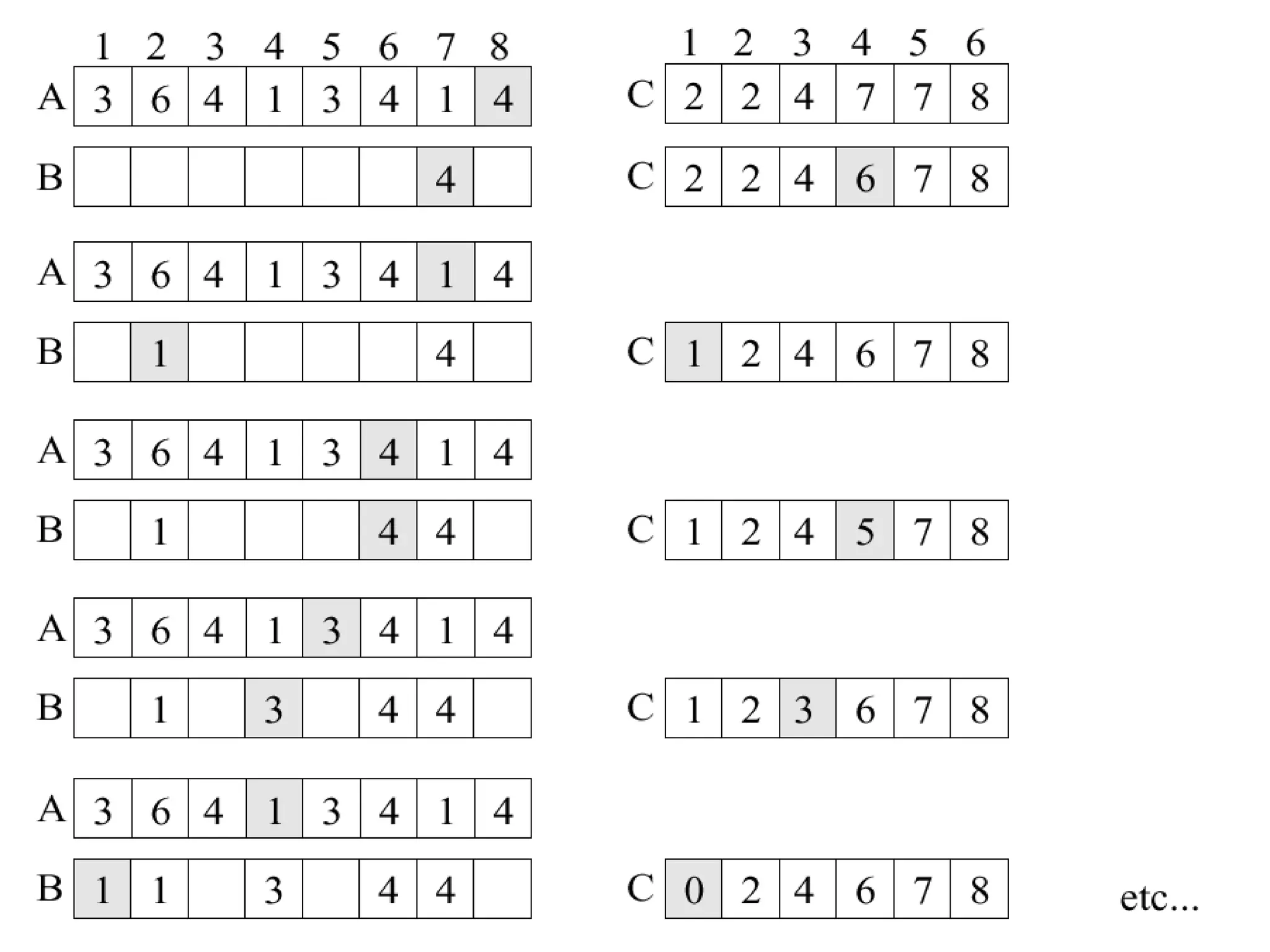
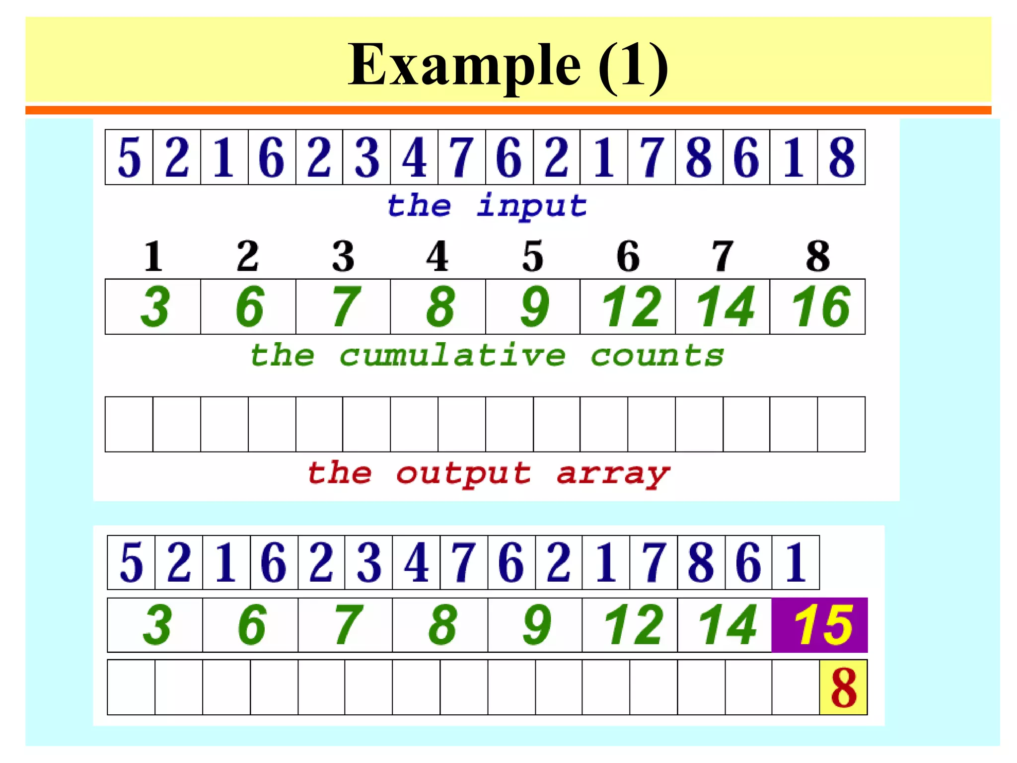
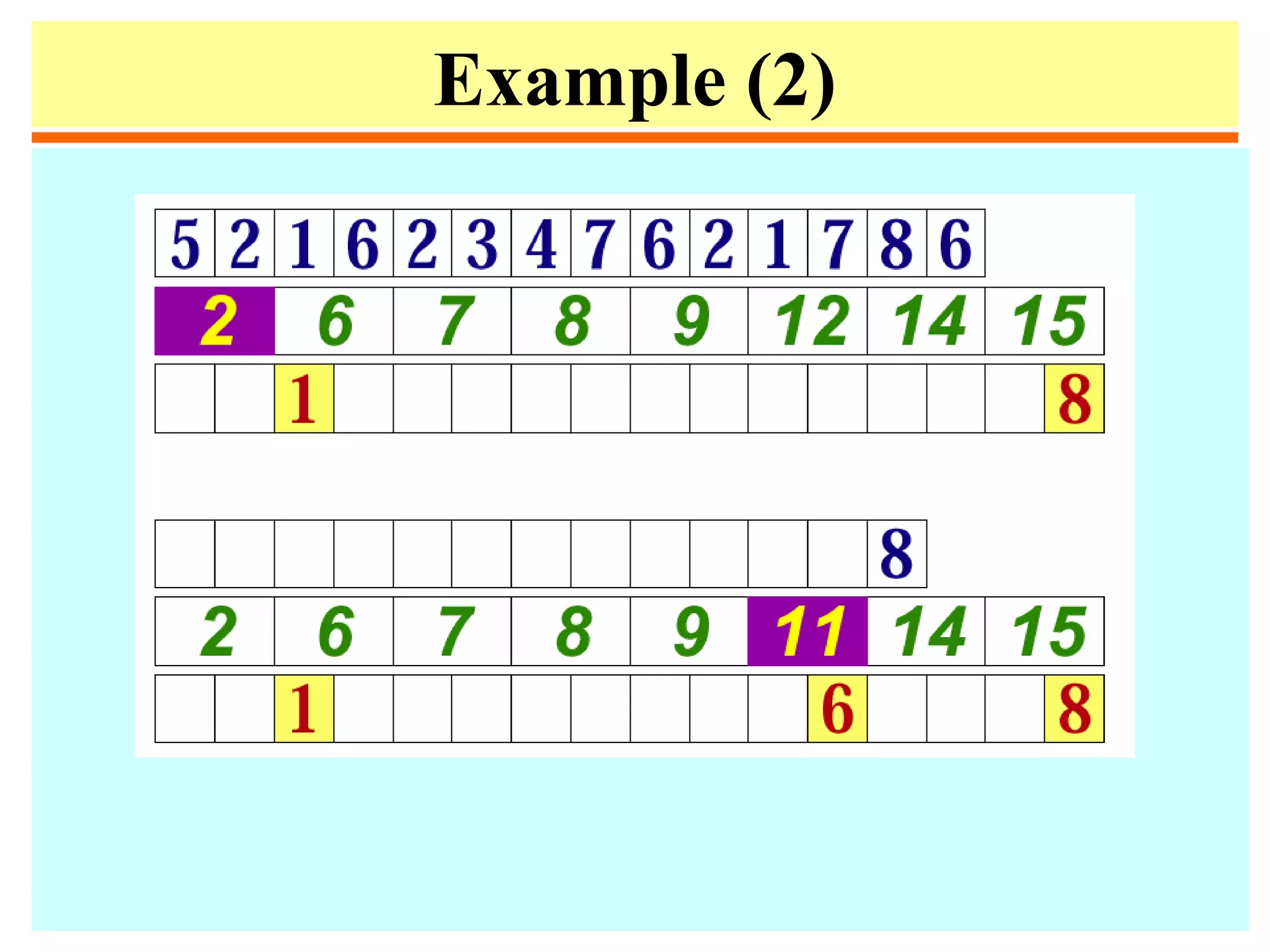
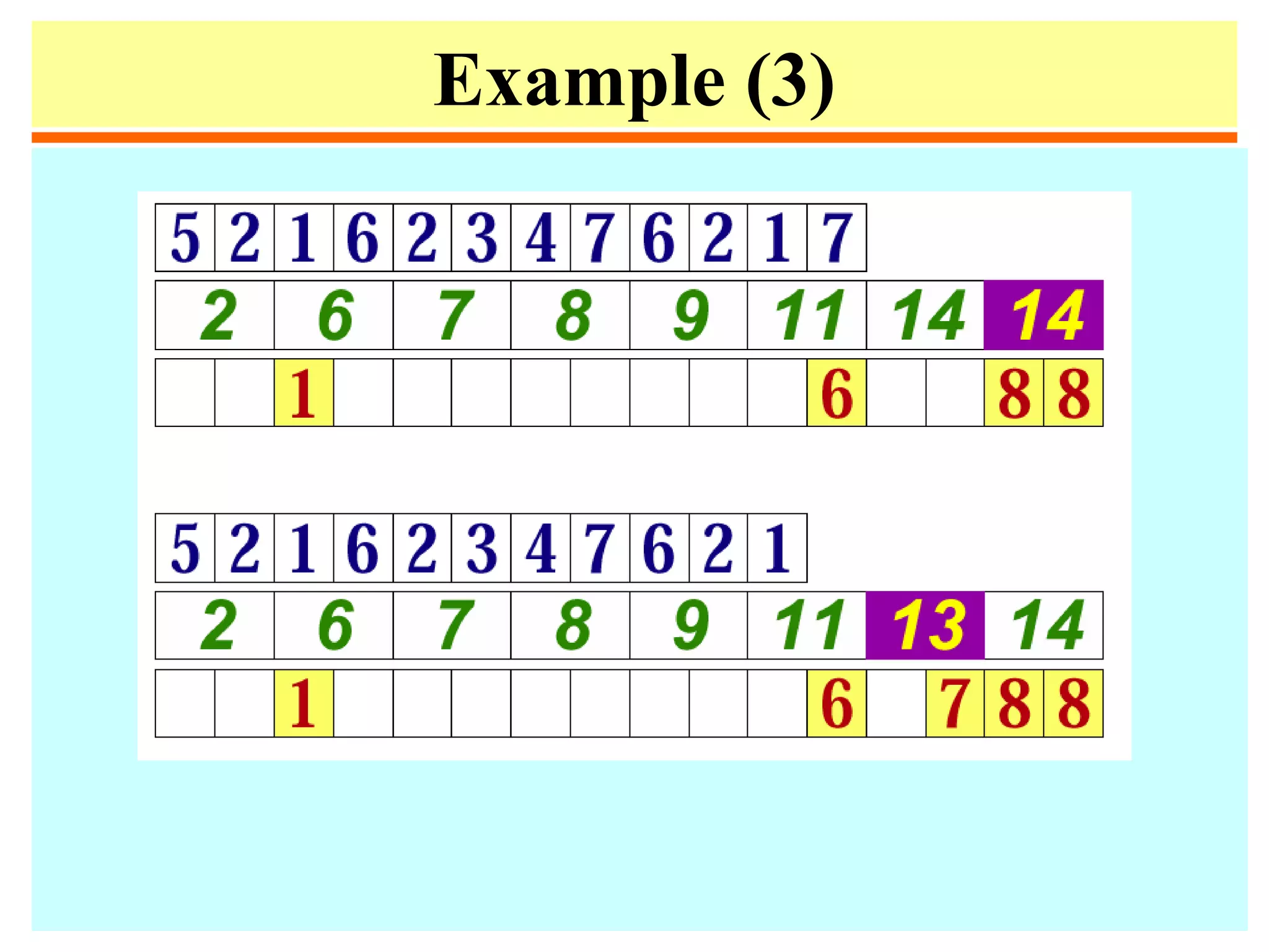
![Distribution counting
• Sort a file of n records whose keys are distinct integers
between 1 and n. Can be done by
for i := 1 to n do t[a[i]] := i.
• Sort a file of n records whose keys are integers between
0 and m-1.
1. for j := 0 to m-1 do count[j] := 0;
2. for i := 1 to n do count[a[i]] := count[a[i]] + 1;
3. for j := 1 to m -1 do count[j] := count[j-1] + count[j];
4. for i := n downto 1 do
begin t[count[a[i]]] := a [i];
count[a[i]] := count[a[i]] -1
end;
5. for i := 1 to n do a[i] := t[i];](https://image.slidesharecdn.com/a13-sorting-150613071621-lva1-app6892/75/sorting-14-2048.jpg)
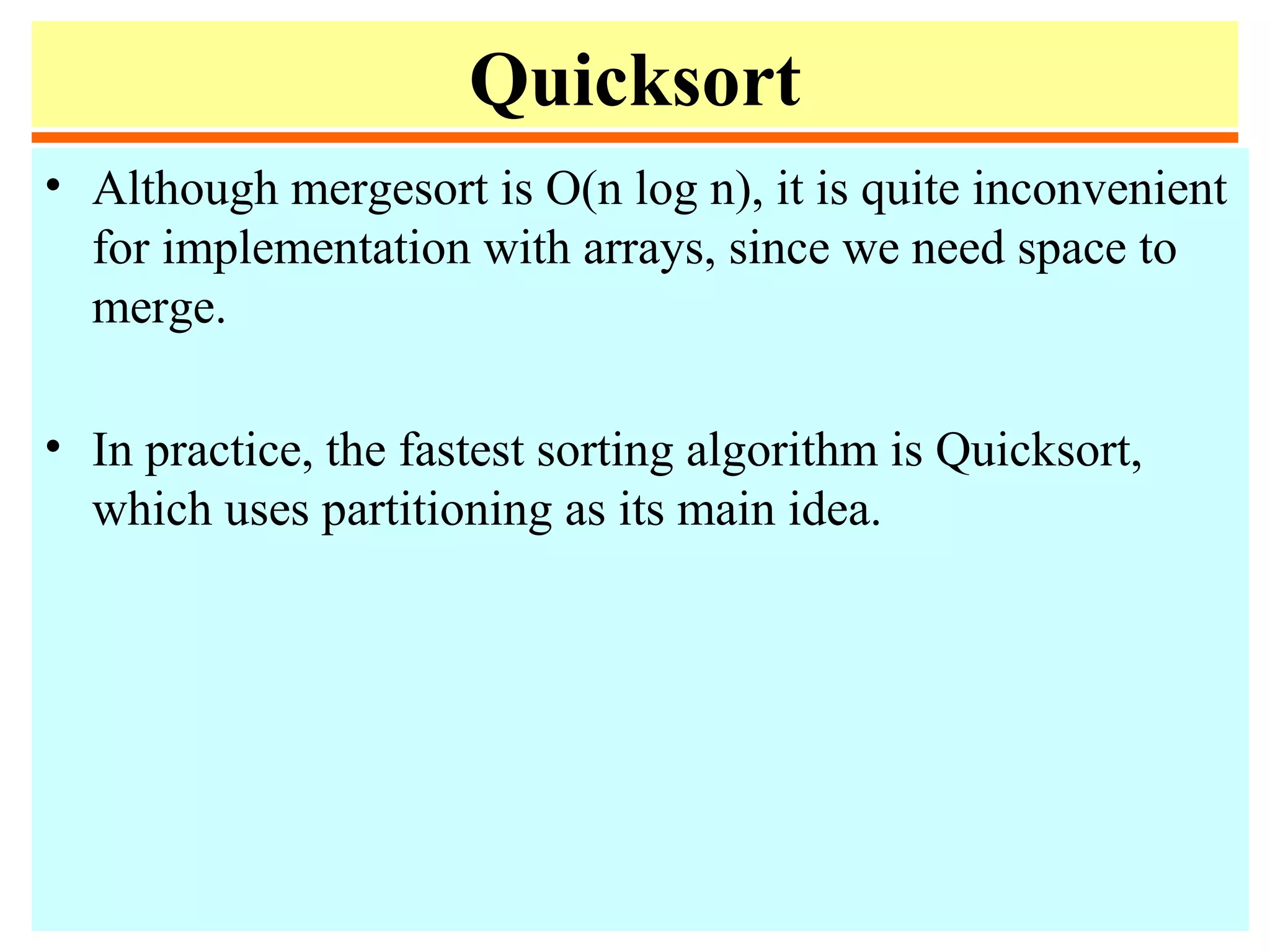
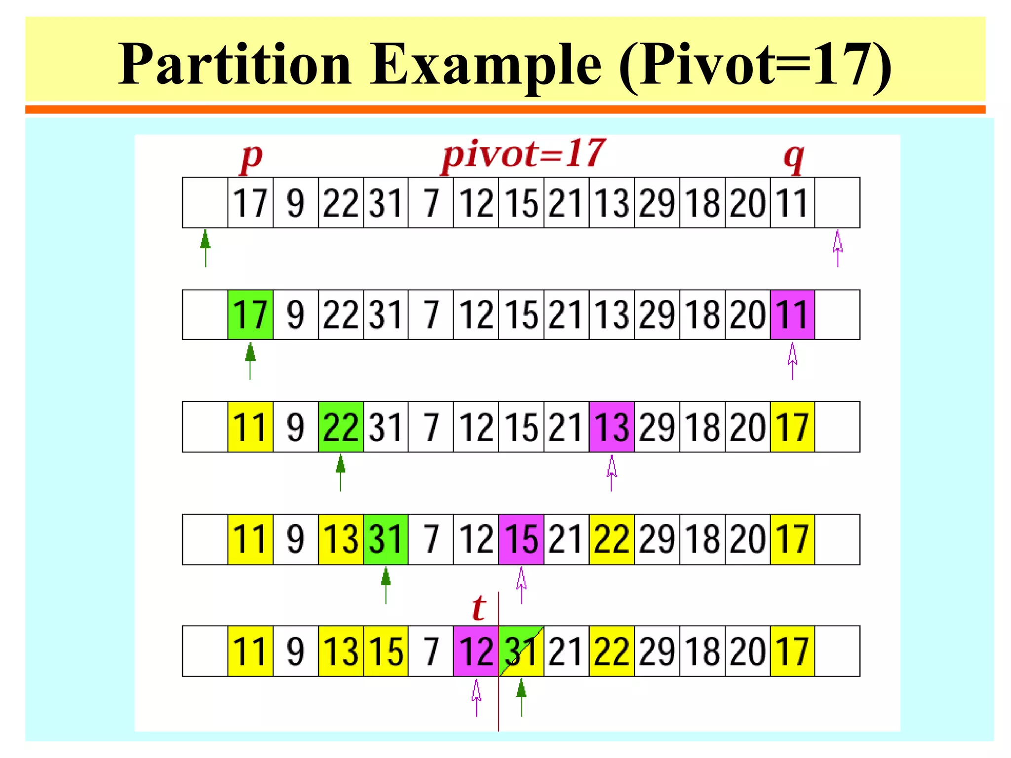
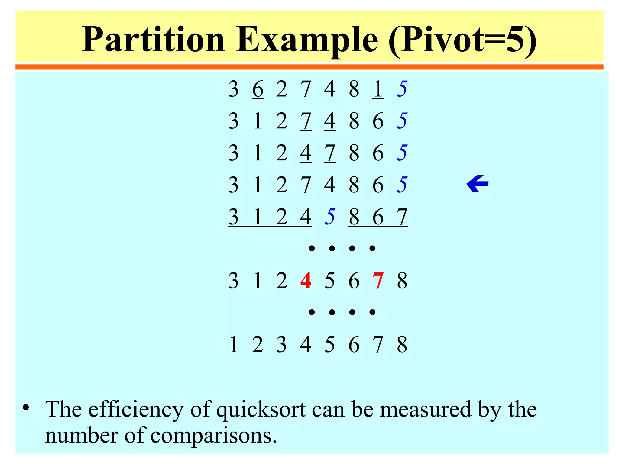
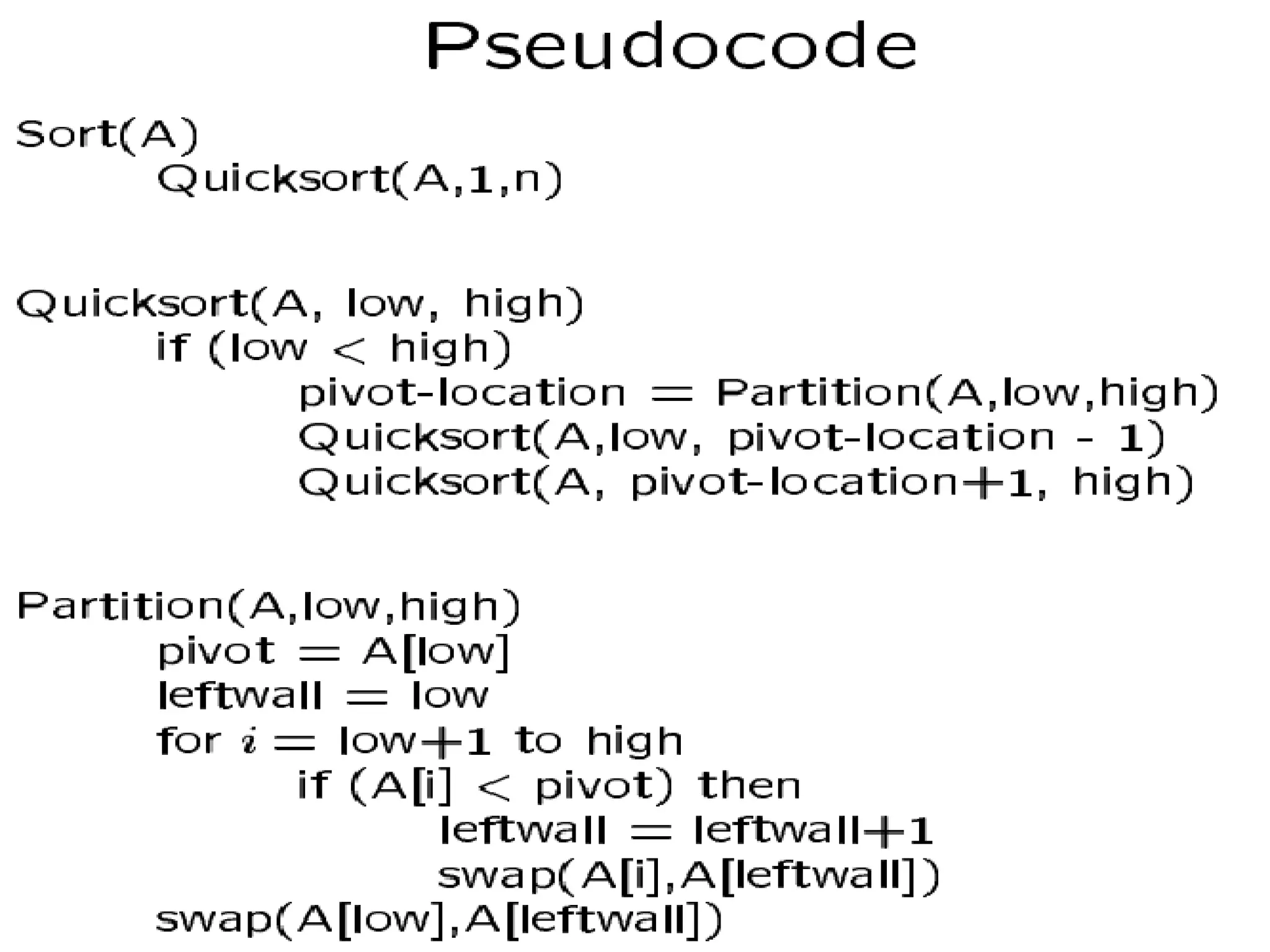
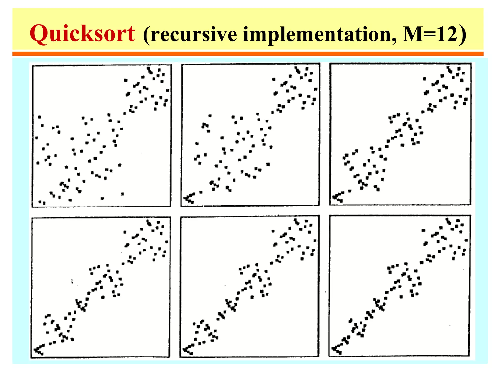
![Quicksort
• Quicksort is a simple divide-and-conquer sorting
algorithm that practically outperforms Heapsort.
• In order to sort A[p..r] do the following:
– Divide: rearrange the elements and generate two
subarrays A[p..q] and A[q+1..r] so that every element
in A[p..q] is at most every element in A[q+1..r];
– Conquer: recursively sort the two subarrays;
– Combine: nothing special is necessary.
• In order to partition, choose u = A[p] as a pivot, and
move everything < u to the left and everything > u to the
right.](https://image.slidesharecdn.com/a13-sorting-150613071621-lva1-app6892/75/sorting-26-2048.jpg)
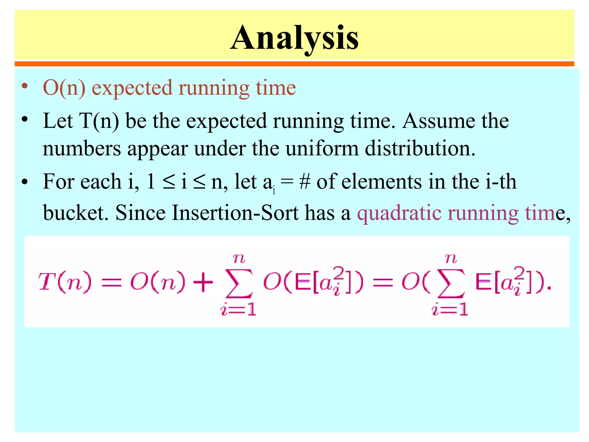
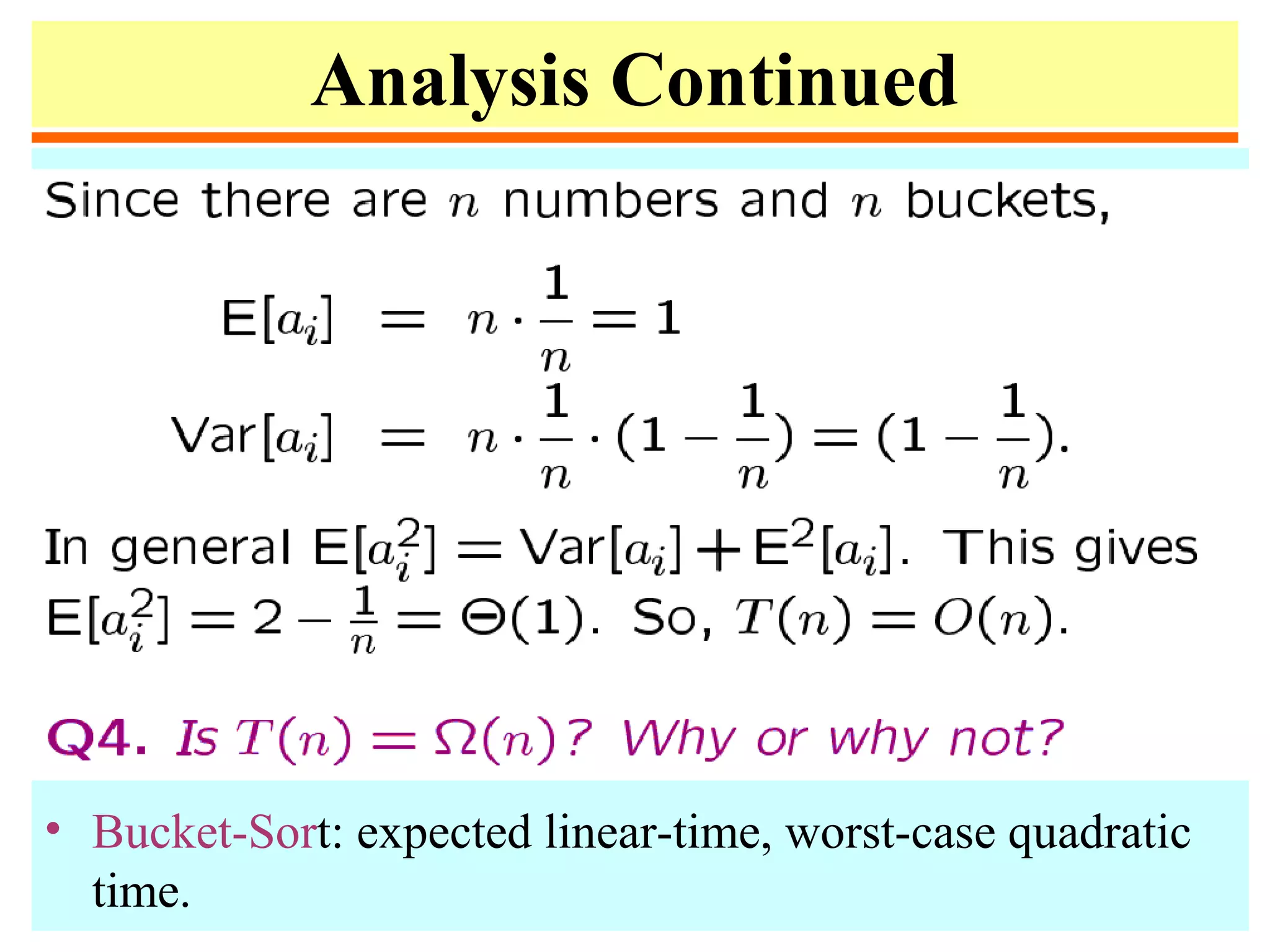
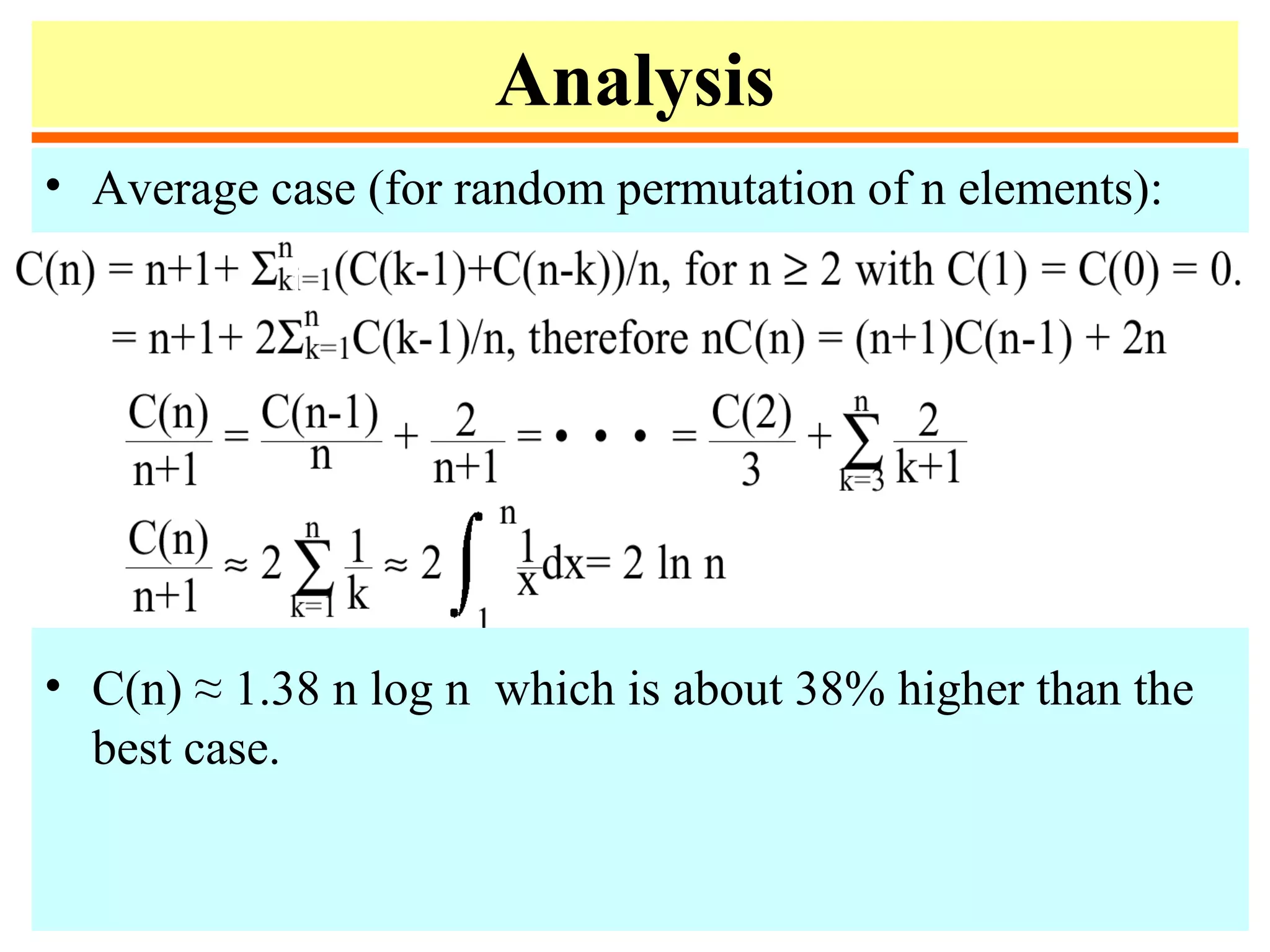
![Analysis
• Worst-case: If A[1..n] is already sorted, then Partition
splits A[1..n] into A[1] and A[2..n] without changing the
order. If that happens, the running time C(n) satisfies:
C(n) = C(1) + C(n –1) + Θ(n) = Θ(n2
)
• Best case: Partition keeps splitting the subarrays into
halves. If that happens, the running time C(n) satisfies:
C(n) ≈ 2 C(n/2) + Θ(n) = Θ(n log n)](https://image.slidesharecdn.com/a13-sorting-150613071621-lva1-app6892/75/sorting-31-2048.jpg)
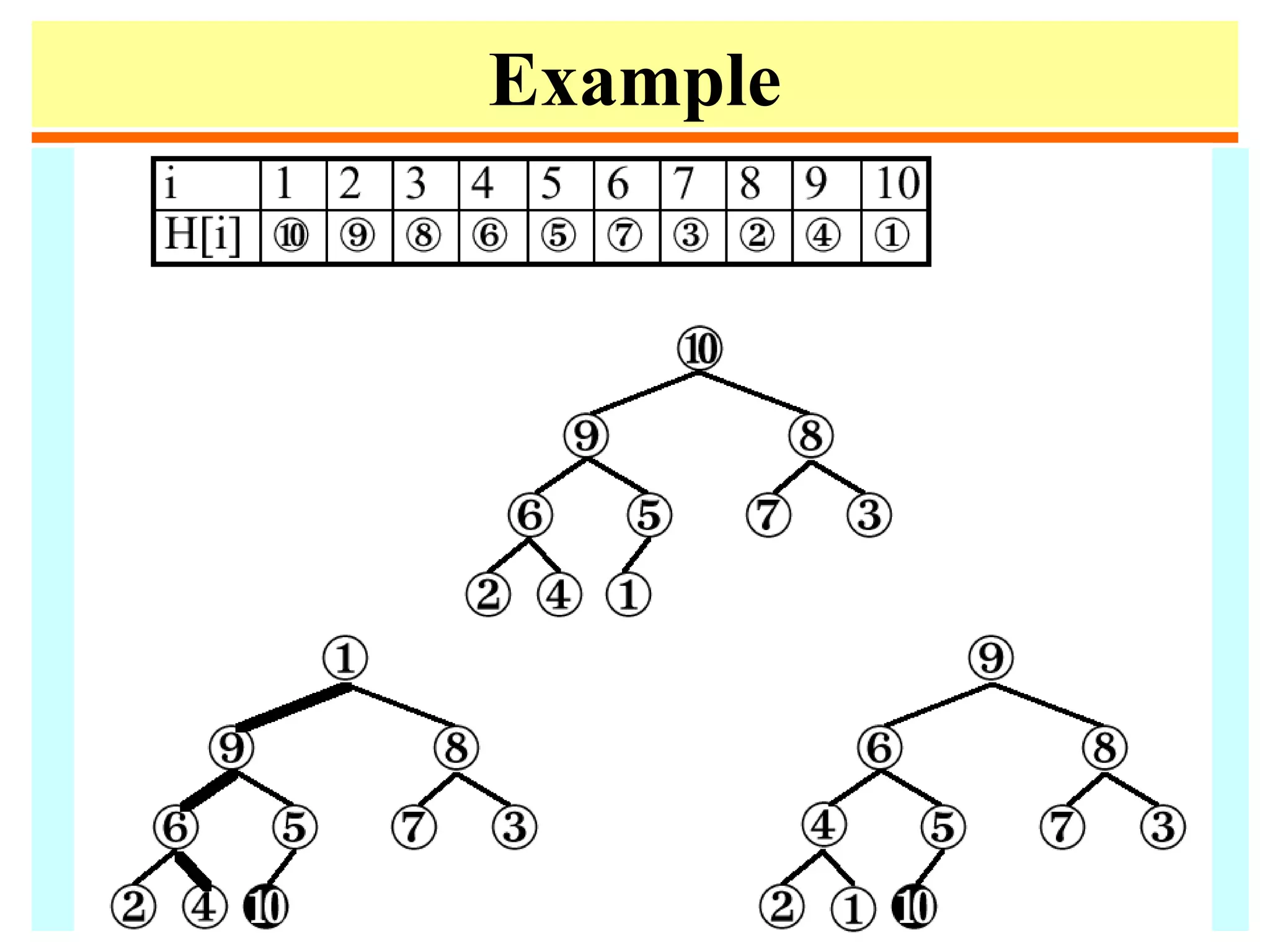
![Example
• The following heap corresponds to the array
A[1..10]: 16, 14, 10, 8, 7, 9, 3, 2, 4, 1](https://image.slidesharecdn.com/a13-sorting-150613071621-lva1-app6892/75/sorting-37-2048.jpg)
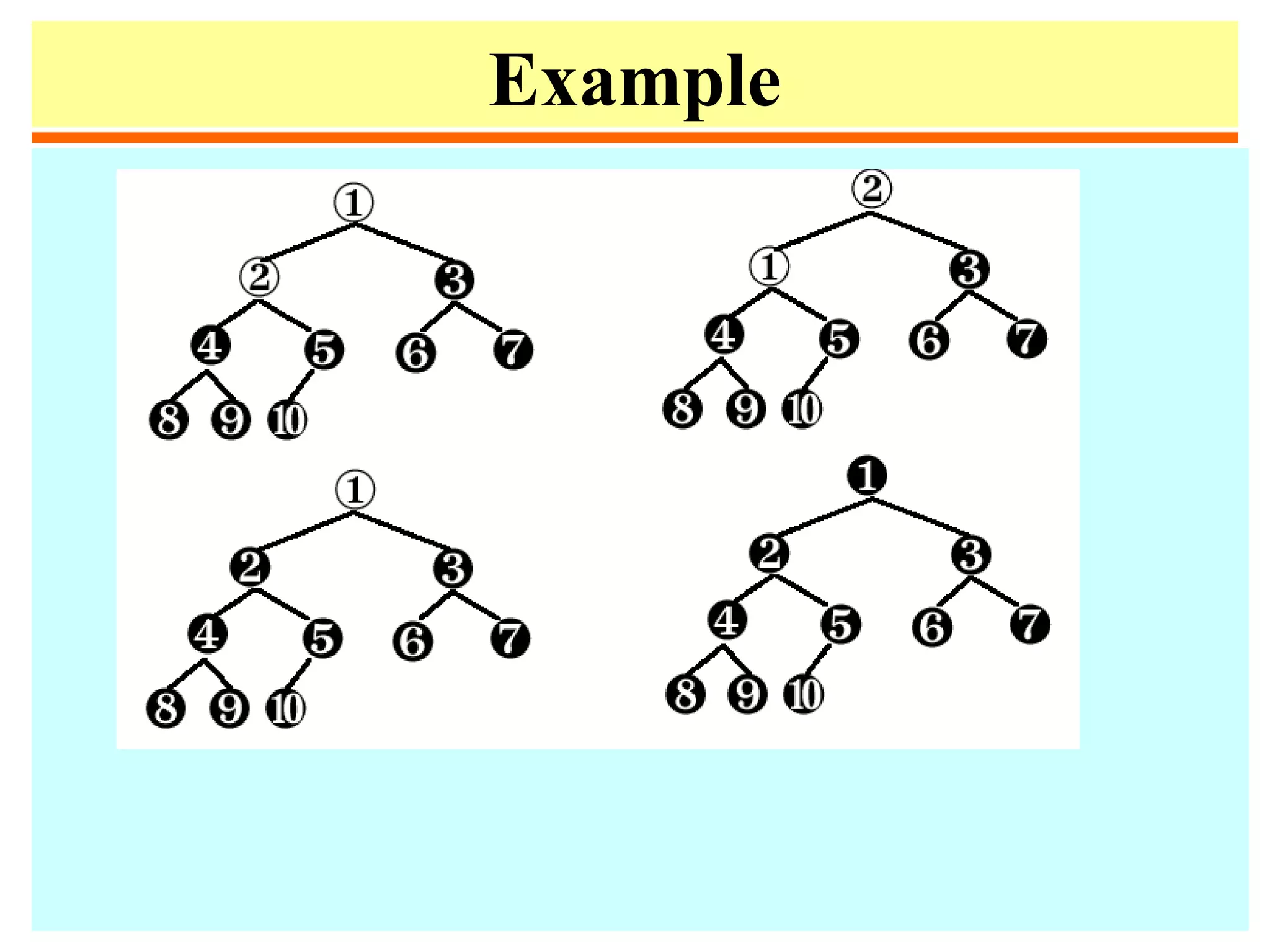
![Heapify
• Heapify at node i: looks at A[i] and A[2i] and A[2i + 1],
the values at the children of i. If the heap-property does
not hold w.r.t. i, exchange A[i] with the larger of A[2i]
and A[2i+1], and recurse on the child with respect to
which exchange took place.
• The number of exchanges is at most the height of the
node, i.e., O(log n).](https://image.slidesharecdn.com/a13-sorting-150613071621-lva1-app6892/75/sorting-38-2048.jpg)
![Pseudocode
1. Heapify(A,i)
2. left = 2i
3. right = 2i +1
4. if (left ≤ n) and(A[left] > A[i])
5. then max = left
6. else max = i
7. if (right ≤ n) and (A(right] > A[max])
8. then max = right
9. if (max ≠ i)
10. then swap(A[i], A[max])
11. Heapify(A, max)](https://image.slidesharecdn.com/a13-sorting-150613071621-lva1-app6892/75/sorting-39-2048.jpg)

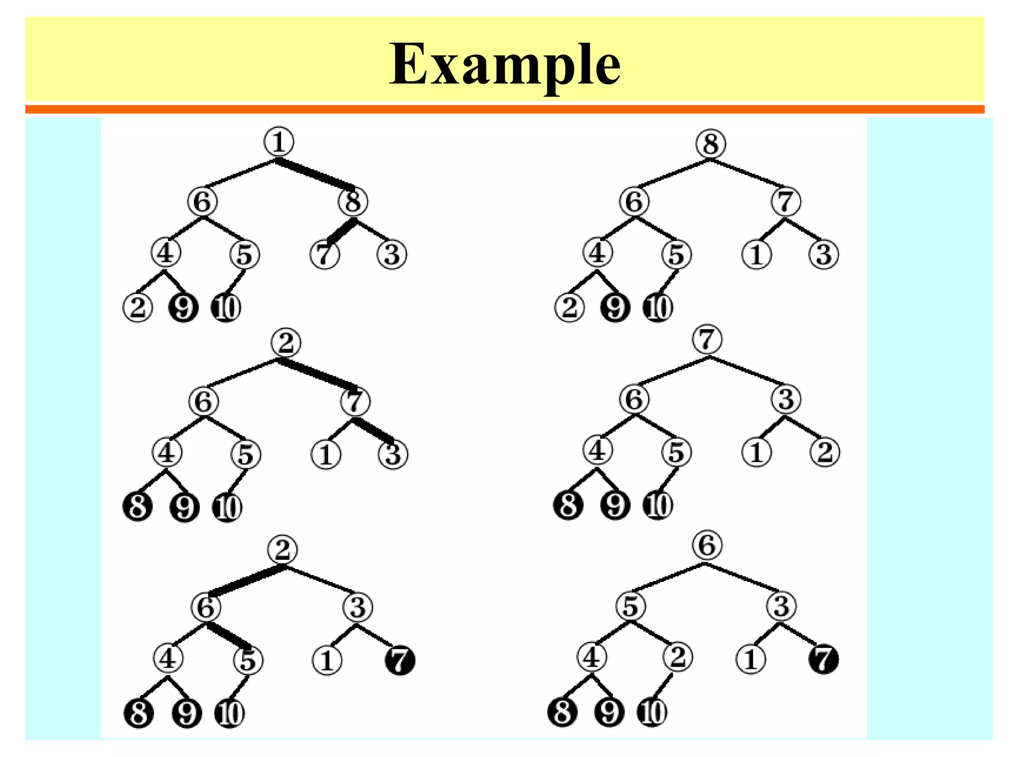
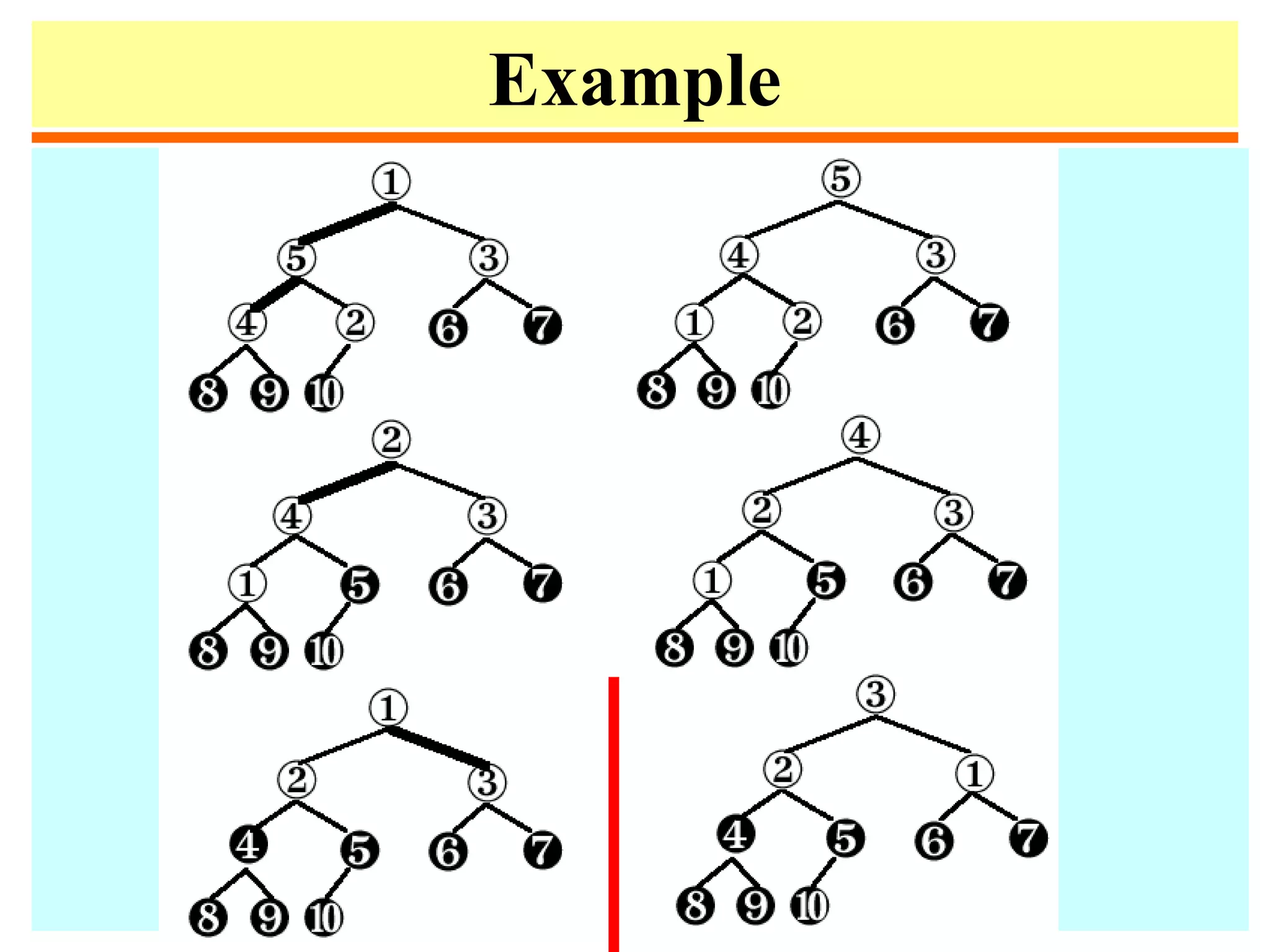
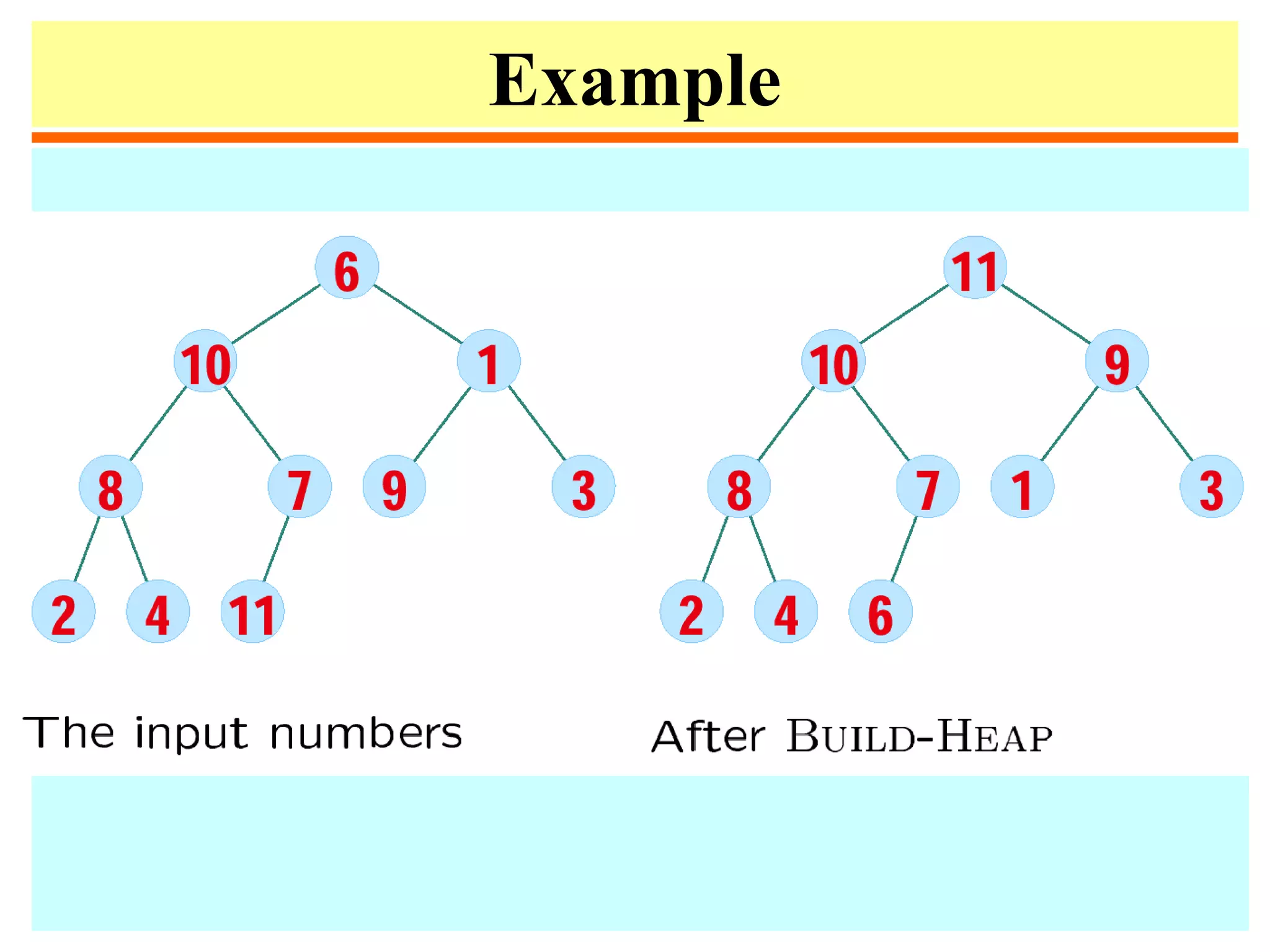
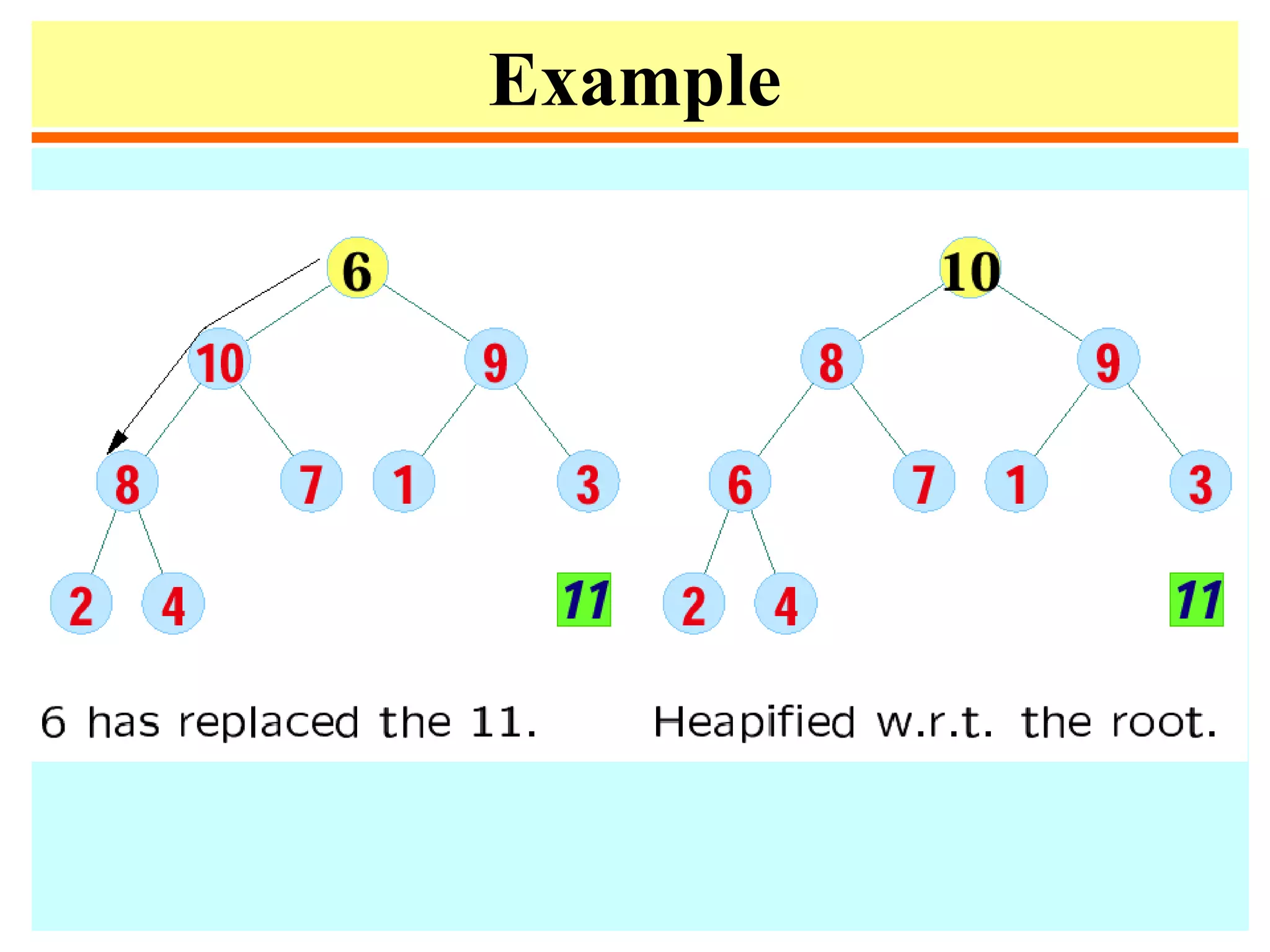
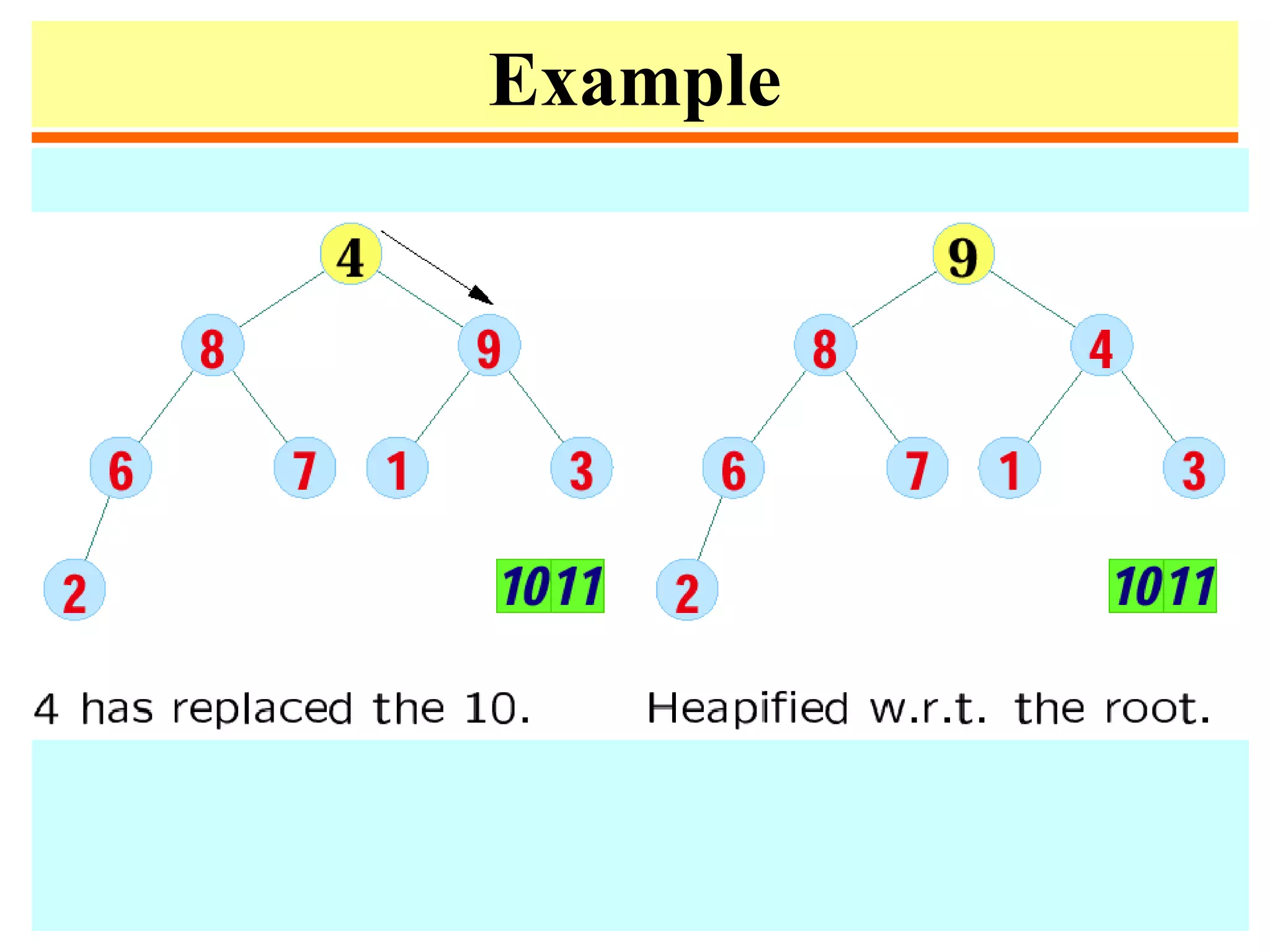
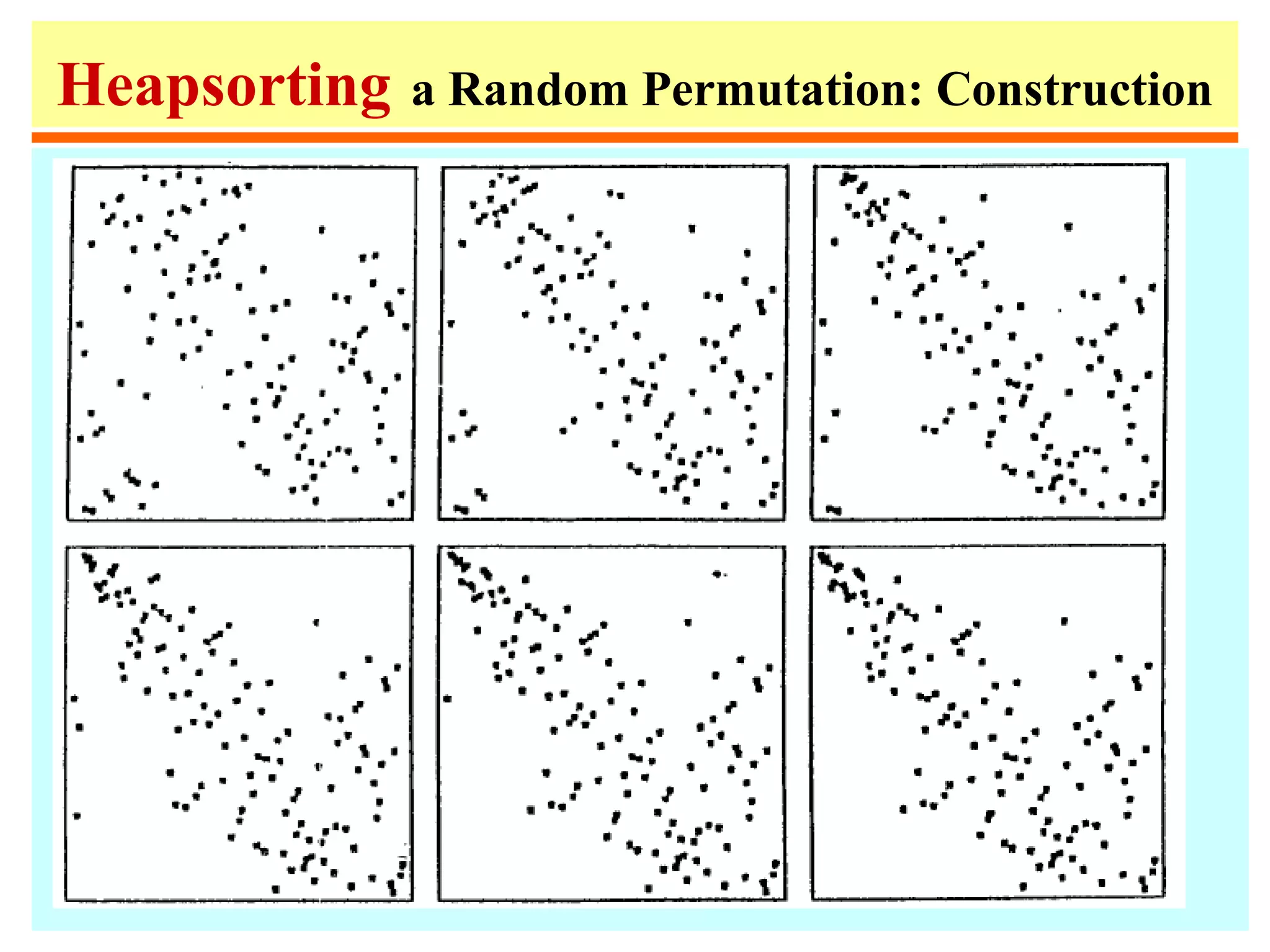
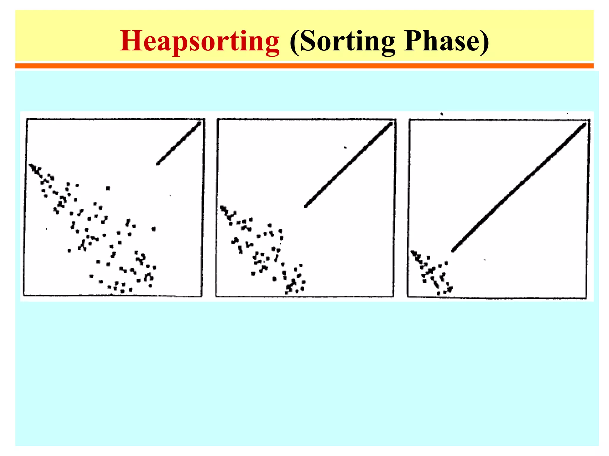
![Heapsort
1. procedure heapsort;
2. var k, t:integer;
3. begin
4. m := n;
5. for i := m div 2 downto 1 do heapify(i);
6. repeat swap(a[1],a[m]);
7. m:=m-1;
8. heapify(1)
9. until m ≤ 1;
10. end;](https://image.slidesharecdn.com/a13-sorting-150613071621-lva1-app6892/75/sorting-46-2048.jpg)
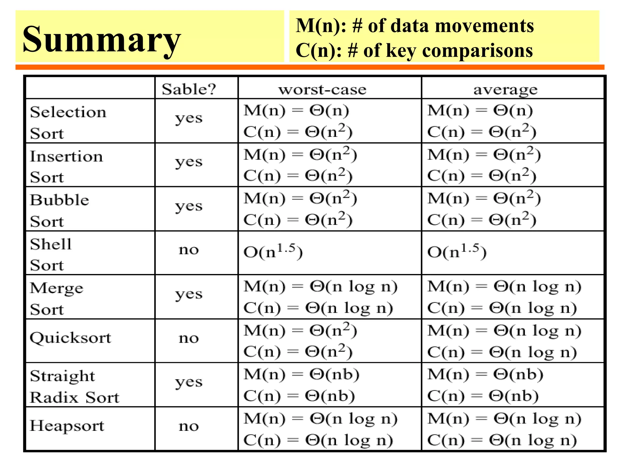

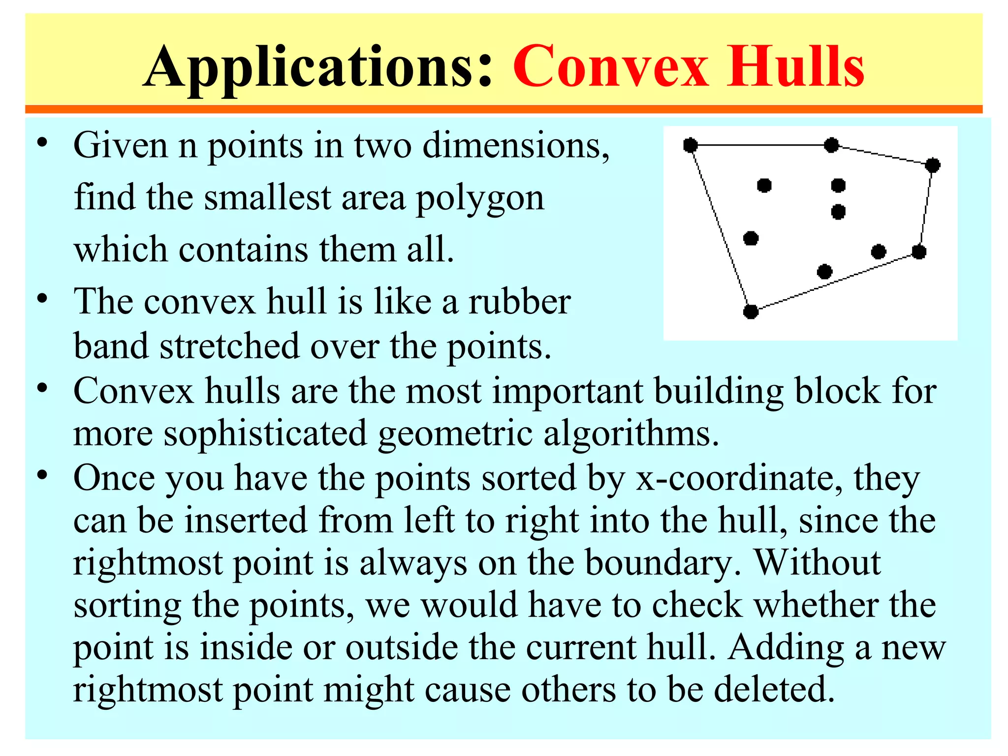
The document discusses sorting algorithms. It defines sorting as arranging a list of records in a certain order based on their keys. Some key points made: - Sorting is important as it enables efficient searching and other tasks. Common sorting algorithms include selection sort, insertion sort, mergesort, quicksort, and heapsort. - The complexity of sorting in general is Θ(n log n) but some special cases allow linear time sorting. Internal sorting happens in memory while external sorting handles data too large for memory. - Applications of sorting include searching, finding closest pairs of numbers, checking for duplicates, and calculating frequency distributions. Sorting also enables efficient algorithms for computing medians, convex hulls, and


![UNIT V Searching Sorting Hashing Techniques [Autosaved].pptx](https://cdn.slidesharecdn.com/ss_thumbnails/unitvsearchingsortinghashingtechniquesautosaved-241014040608-74caa0f6-thumbnail.jpg?width=640&height=640&fit=bounds)

![UNIT V Searching Sorting Hashing Techniques [Autosaved].pptx](https://cdn.slidesharecdn.com/ss_thumbnails/unitvsearchingsortinghashingtechniquesautosaved-241126054304-95a69c51-thumbnail.jpg?width=640&height=640&fit=bounds)