Downloaded 30 times


![ Sorting is among the most basic problems in algorithm design.
Sorting is important because it is often the first step in more complex
algorithms.
Sorting is to take an unordered set of comparable items and arrange them
in some order.
That is, sorting is a process of arranging the items in a list in some order
that is either ascending or descending order.
Let a[n] be an array of n elements a0,a1,a2,a3........,an-1 in memory. The
sorting of the array a[n] means arranging the content of a[n] in either
increasing or decreasing order.
i.e. a0<=a1<=a2<=a3<.=.......<=an-1
Introduction
3
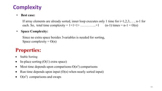
• Efficient sorting is important for optimizing the use of other algorithms
(such as search and merge algorithms) that require sorted lists to work
correctly.](https://image.slidesharecdn.com/unit-7sorting-171201035431/85/Unit-7-sorting-3-320.jpg)
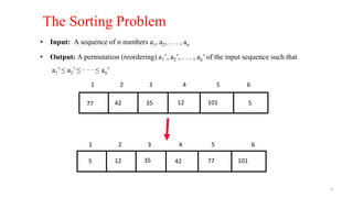

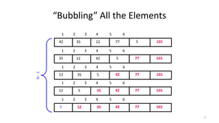
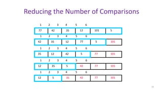
![Bubble Sort
• The basic idea of this sort is to pass through the array sequentially several
times.
• Each pass consists of comparing each element in the array with its successor
(for example a[i] with a[i + 1]) and interchanging the two elements if they
are not in the proper order.
• After each pass an element is placed in its proper place and is not considered
in succeeding passes.
7](https://image.slidesharecdn.com/unit-7sorting-171201035431/85/Unit-7-sorting-7-320.jpg)

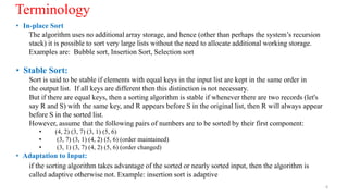
![Algorithm
BubbleSort(A, n)
{
for(i = 0; i <n-1; i++)
{
for(j = 0; j < n-i-1; j++)
{
if(A[j] > A[j+1])
{
temp = A[j];
A[j] = A[j+1];
A[j+1] = temp;
}
}
}
}
19](https://image.slidesharecdn.com/unit-7sorting-171201035431/85/Unit-7-sorting-19-320.jpg)
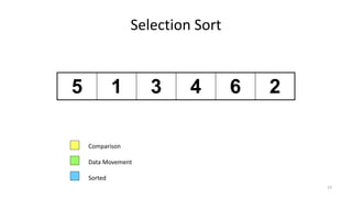
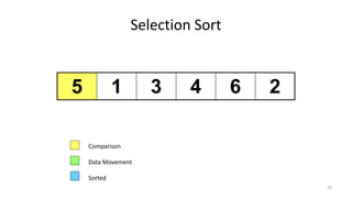
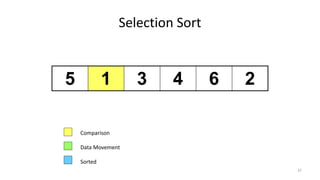
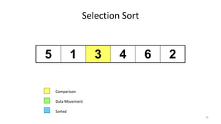
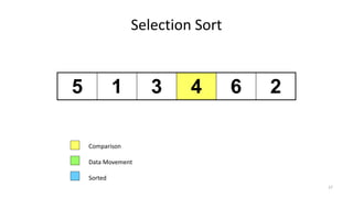
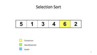
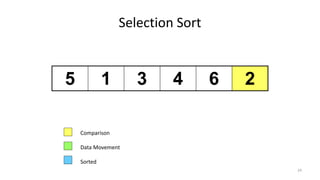
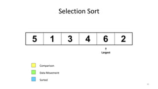
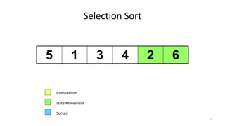
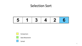
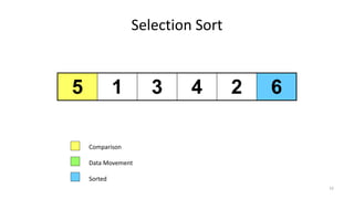
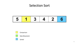
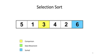
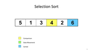
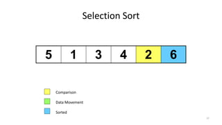
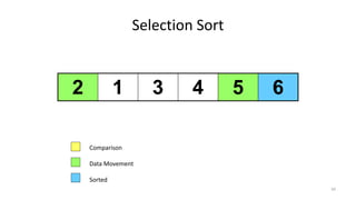
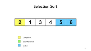
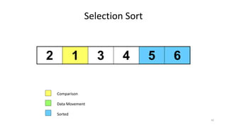
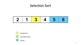
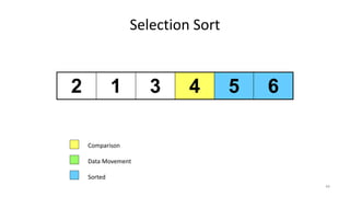
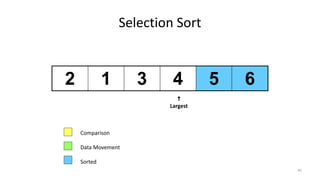
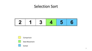
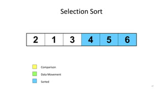
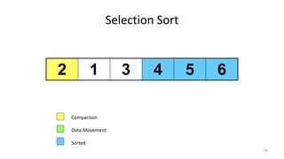
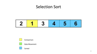
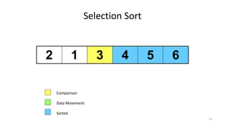
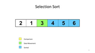
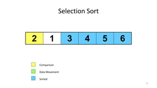
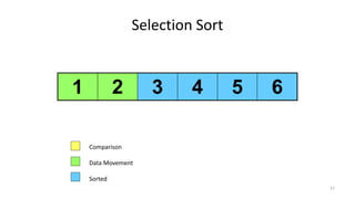
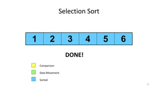
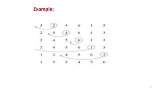
![Selection Sort
• Idea:
Find the least (or greatest) value in the array, swap it into the leftmost(or
rightmost)component (where it belongs), and then forget the leftmost
component. Do this repeatedly.
• Process:
Let a[n] be a linear array of n elements. The selection sort works as follows:
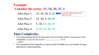
Pass 1: Find the location loc of the maximum element in the list of n
elements a[0], a[1], a[2], a[3], …......,a[n-1] and then interchange a[loc] and
a[n-1].
Pass 2: Find the location loc of the max element in the sub-list of n-1
elements a[0], a[1], a[2], a[3], …......,a[n-2] and then interchange a[loc] and
a[n-2].
Continue in the same way. Finally, we will get the sorted list:
a[0]<=a[1]<= a[2]<=a[3]<= .....<= a[n-1]. 22](https://image.slidesharecdn.com/unit-7sorting-171201035431/85/Unit-7-sorting-22-320.jpg)


![Algorithm:
SelectionSort(A)
{
for( i = 0; i < n-1 ; i++)
{
max = A[0];
loc=0;
for ( j = 1; j < =n-1-i ; j++)
{
if (A[j] > max)
{
max = A[j];
loc=j;
}
}
if( n-1-i!=loc)
swap(A[n-1-i],A[loc]);
}
}
59](https://image.slidesharecdn.com/unit-7sorting-171201035431/85/Unit-7-sorting-59-320.jpg)
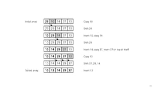
![• Idea: Like sorting a hand of playing cards start with an empty left hand and the cards
facing down on the table. Remove one card at a time from the table, Compare it with
each of the cards already in the hand, from right to left and insert it into the correct
position in the left hand. The cards held in the left hand are sorted.
• Suppose an array a[n] with n elements. The insertion sort works as follows:
• Pass 1: a[0] by itself is trivially sorted.
• Pass 2: a[1] is inserted either before or after a[0] so that a[0], a[1] is sorted.
• Pass 3: a[2] is inserted into its proper place in a[0],a[1] that is before a[0], between a[0]
and a[1], or after a[1] so that a[0],a[1],a[2] is sorted.
.......................................
• Pass N: a[n-1] is inserted into its proper place in a[0],a[1],a[2],........,a[n-2] so that
a[0],a[1],a[2],............,a[n-1] is sorted with n elements.
62
Insertion Sort](https://image.slidesharecdn.com/unit-7sorting-171201035431/85/Unit-7-sorting-62-320.jpg)
![64
InsertionSort(A)
{
for( i = 1;i < n ;i++)
{
temp = A[i]
for ( j = i -1; j >= 0; j--)
{
if(A[j] > temp )
A[j+1] = A[j];
}
A[j+1] = temp;
}
}
Algorithm:](https://image.slidesharecdn.com/unit-7sorting-171201035431/85/Unit-7-sorting-64-320.jpg)
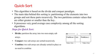
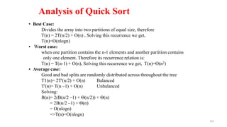
![68
Quicksort Algorithm
To sort a[left...right]:
1. if left < right:
1.1. Partition a[left...right] such that: all a[left...p-1] are less
than a[p], and all a[p+1...right] are >= a[p]
1.2. Quicksort a[left...p-1]
1.3. Quicksort a[p+1...right]
2. Terminate
p
numbers less
than p
numbers greater than or
equal to p
p](https://image.slidesharecdn.com/unit-7sorting-171201035431/85/Unit-7-sorting-68-320.jpg)
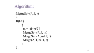
![70
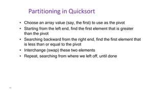
Partitioning
To partition a[left...right]:
1. Set pivot = a[left], l = left + 1, r = right;
2. while l < r, do
2.1. while l < right & a[l] <= pivot , set l = l + 1
2.2. while r > left & a[r] > pivot , set r = r - 1
2.3. if l < r, swap a[l] and a[r]
3. Set a[left] = a[r], a[r] = pivot
4. Terminate](https://image.slidesharecdn.com/unit-7sorting-171201035431/85/Unit-7-sorting-70-320.jpg)
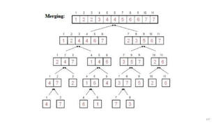
![72
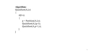
Partition(A,l,r)
{
x =l;
y =r ;
p = A[l];
while(x<y)
{
while(A[x] <= p)
x++;
while(A[y] >p)
y--;
if(x<y)
swap(A[x],A[y]);
}
A[l] = A[y];
A[y] = p;
return y; //return position of pivot
}](https://image.slidesharecdn.com/unit-7sorting-171201035431/85/Unit-7-sorting-72-320.jpg)
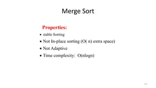
![73
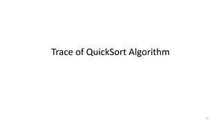
Example: a[]={5, 3, 2, 6, 4, 1, 3, 7}
(1 3 2 3 4) 5 (6 7)
and continue this process for each sub-arrays and finally we get a sorted array.](https://image.slidesharecdn.com/unit-7sorting-171201035431/85/Unit-7-sorting-73-320.jpg)
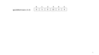
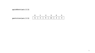
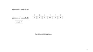
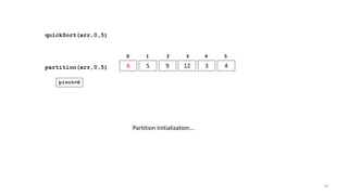
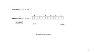
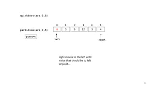
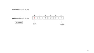
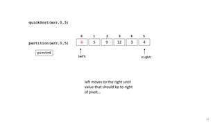
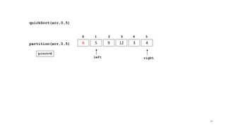
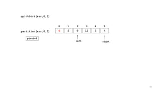

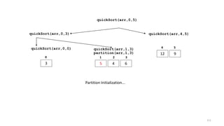
![quickSort(arr,0,5)
6 5 4 12 3 9
0 1 2 3 4 5
partition(arr,0,5)
left right
pivot=6
swap arr[left] and arr[right]
87](https://image.slidesharecdn.com/unit-7sorting-171201035431/85/Unit-7-sorting-87-320.jpg)
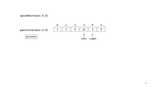
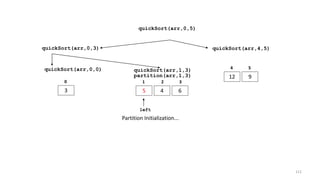
![quickSort(arr,0,5)
6 5 4 3 12 9
0 1 2 3 4 5
partition(arr,0,5)
left
right
pivot=6
right & left CROSS!!!
1 - Swap pivot and arr[right]
89](https://image.slidesharecdn.com/unit-7sorting-171201035431/85/Unit-7-sorting-89-320.jpg)
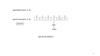
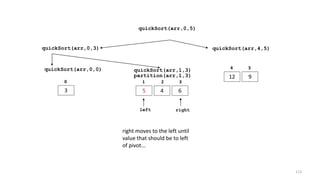
![quickSort(arr,0,5)
3 5 4 6 12 9
0 1 2 3 4 5
partition(arr,0,5)
left
right
pivot=6
right & left CROSS!!!
1 - Swap pivot and arr[right]
90](https://image.slidesharecdn.com/unit-7sorting-171201035431/85/Unit-7-sorting-90-320.jpg)
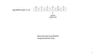
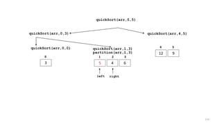
![quickSort(arr,0,5)
3 5 4 6 12 9
0 1 2 3 4 5
partition(arr,0,5)
left
right
pivot=6
right & left CROSS!!!
1 - Swap pivot and arr[right]
2 - Return new location of pivot to caller
return 3
91](https://image.slidesharecdn.com/unit-7sorting-171201035431/85/Unit-7-sorting-91-320.jpg)
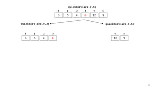
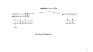
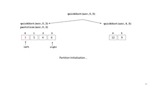
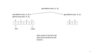
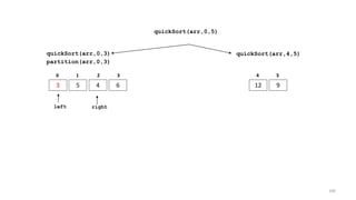
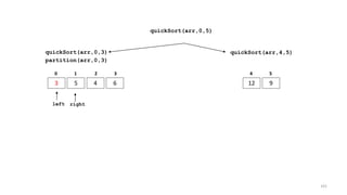
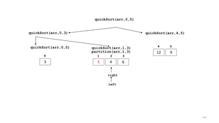
![quickSort(arr,0,3)
3 5 4 6
0 1 2 3
quickSort(arr,4,5)
12 9
4 5
partition(arr,0,3)
left
right
right & left CROSS!!!
1 - Swap pivot and arr[right]
quickSort(arr,0,5)
104](https://image.slidesharecdn.com/unit-7sorting-171201035431/85/Unit-7-sorting-104-320.jpg)
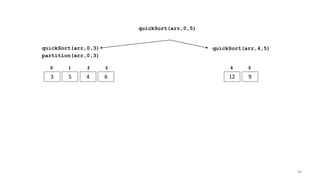
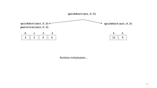
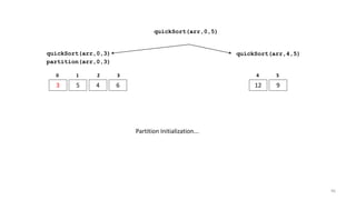
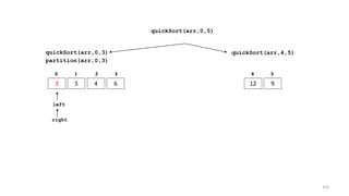
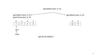
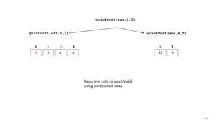
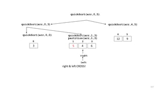
![quickSort(arr,0,3)
3 5 4 6
0 1 2 3
quickSort(arr,4,5)
12 9
4 5
partition(arr,0,3)
left
right
right & left CROSS!!!
1 - Swap pivot and arr[right]
right & left CROSS!!!
1 - Swap pivot and arr[right]
2 - Return new location of pivot to caller
return 0
quickSort(arr,0,5)
105](https://image.slidesharecdn.com/unit-7sorting-171201035431/85/Unit-7-sorting-105-320.jpg)
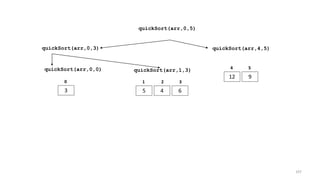
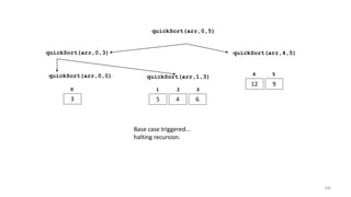
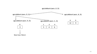

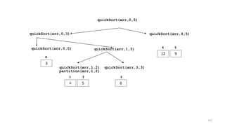
![quickSort(arr,0,3) quickSort(arr,4,5)
12 9
4 5
quickSort(arr,0,5)
quickSort(arr,0,0)
3
0
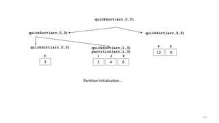
quickSort(arr,1,3)
5 4 6
1 2 3
partition(arr,1,3)
left
right
right & left CROSS!
1- swap pivot and arr[right]
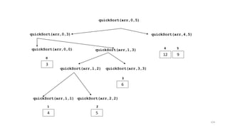
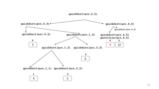
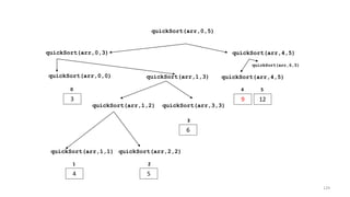
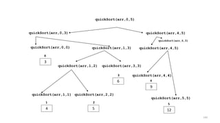
118](https://image.slidesharecdn.com/unit-7sorting-171201035431/85/Unit-7-sorting-118-320.jpg)
![quickSort(arr,0,3) quickSort(arr,4,5)
12 9
4 5
quickSort(arr,0,5)
quickSort(arr,0,0)
3
0
quickSort(arr,1,3)
4 5 6
1 2 3
partition(arr,1,3)
left
right
right & left CROSS!
1- swap pivot and arr[right]
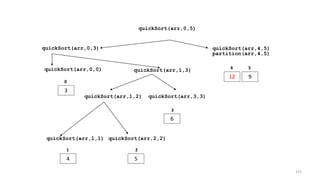
119](https://image.slidesharecdn.com/unit-7sorting-171201035431/85/Unit-7-sorting-119-320.jpg)
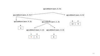
![quickSort(arr,0,3) quickSort(arr,4,5)
12 9
4 5
quickSort(arr,0,5)
quickSort(arr,0,0)
3
0
quickSort(arr,1,3)
4 5 6
1 2 3
partition(arr,1,3)
left
right
right & left CROSS!
1- swap pivot and arr[right]
2 – return new position of pivot
return 2
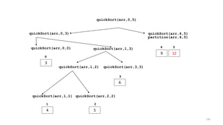
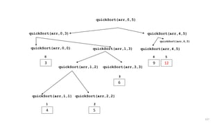
120](https://image.slidesharecdn.com/unit-7sorting-171201035431/85/Unit-7-sorting-120-320.jpg)

![133
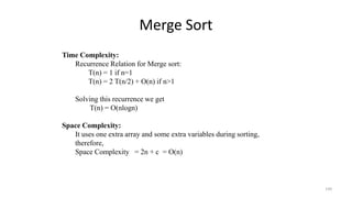
Merge Sort
Merge sort is divide and conquer algorithm. It is recursive algorithm
having three steps. To sort an array A[l . . r]:
• Divide
Divide the n-element sequence to be sorted into two sub-sequences of
n/2 elements
• Conquer
Sort the sub-sequences recursively using merge sort. When the size of
the sequences is 1 there is nothing more to do
•Combine
Merge the two sorted sub-sequences into single sorted array. Keep
track of smallest element in each sorted half and inset smallest of two
elements into auxiliary array. Repeat this until done.](https://image.slidesharecdn.com/unit-7sorting-171201035431/85/Unit-7-sorting-133-320.jpg)
![Merge operation
Merge(A, B, l, m, r)
{
x= l, y=m, k =l;
While(x<m && y<=r)
{
if(A[x] < A[y])
{
B[k] = A[x];
k++; x++;
}
else
{
B[k] = A[y];
k++; y++;
}
} 135
while(x<m)
{
B[k] = A[x];
k++;x++;
}
while(y<=r)
{
B[k] = A[y];
k++; y++;
}
For(i =1;i<=r;i++)
{
A[i] = B[i];
}
} // end of merge](https://image.slidesharecdn.com/unit-7sorting-171201035431/85/Unit-7-sorting-135-320.jpg)
![136
Example: a[]= {4, 7, 2, 6, 1, 4, 7, 3, 5, 2, 6}](https://image.slidesharecdn.com/unit-7sorting-171201035431/85/Unit-7-sorting-136-320.jpg)
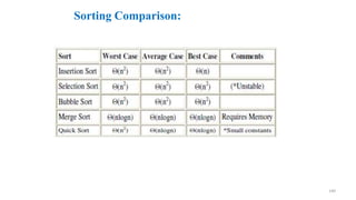


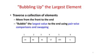
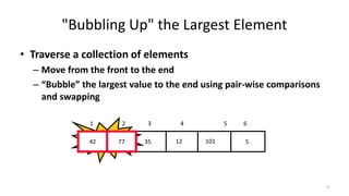
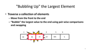
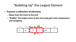
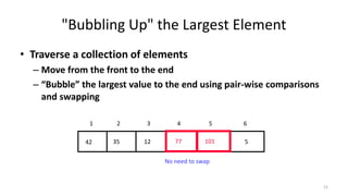
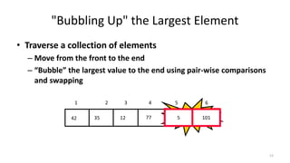
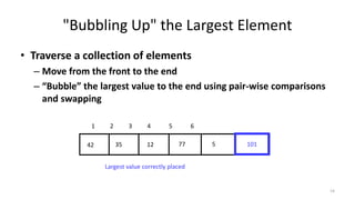
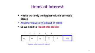
The document discusses various sorting algorithms. It provides an overview of bubble sort, selection sort, and insertion sort. For bubble sort, it explains the process of "bubbling up" the largest element to the end of the array through successive passes. For selection sort, it illustrates the process of finding the largest element and swapping it into the correct position in each pass to sort the array. For insertion sort, it notes that elements are inserted into the sorted portion of the array in the proper position.