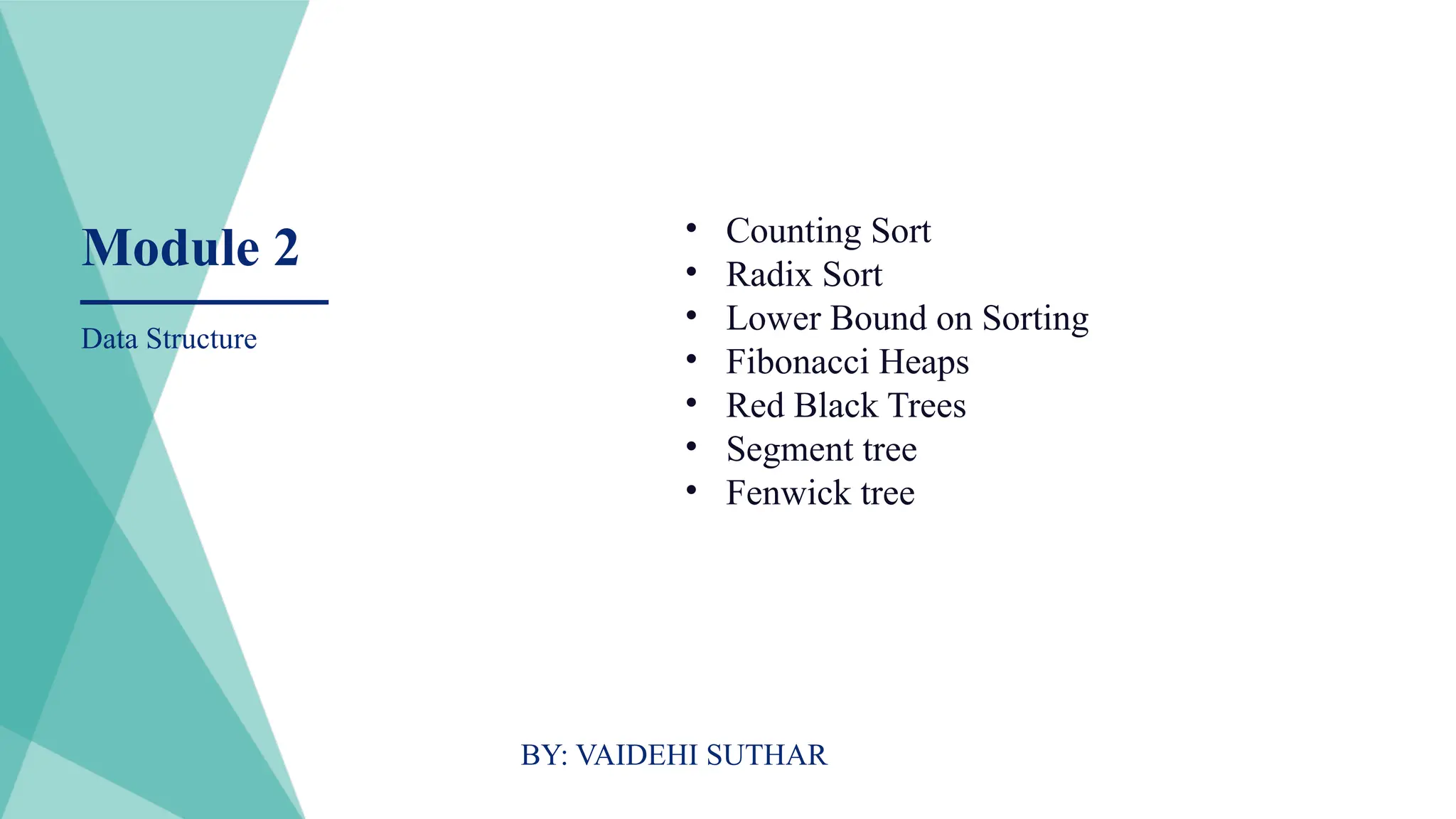
Module 2
Data Structure
•Counting Sort
• Radix Sort
• Lower Bound on Sorting
• Fibonacci Heaps
• Red Black Trees
• Segment tree
• Fenwick tree
BY: VAIDEHI SUTHAR
2.
Counting Sort
• CountingSort is a non-comparison-based sorting
algorithm. [ used to arrange data without comparing
elements directly.]
• It is particularly efficient when the range of input values is
small compared to the number of elements to be sorted.
• The basic idea behind Counting Sort is to count
the frequency of each distinct element in the input array and
use that information to place the elements in their correct
sorted positions.
• For example, for input [1, 4, 3, 2, 2, 1], the output should be
[1, 1, 2, 2, 3, 4].
3.
Working of
Counting Sort
Findout the maximum element
from the given array.
Initialize a countArray[] of
length max+1 with all elements as 0.
This array will be used for storing the occurrences
of the elements of the input array.
countArray[], store the count of each unique
element of the input array at their respective
indices.
Store the cumulative sum or prefix sum of the
elements of the countArray[] by doing
countArray[i] = countArray[i – 1] +
countArray[i].
This will help in placing the elements of the input
array at the correct index in the output array.
Counting Sort
Algorithm:
•Declare anauxiliary array countArray[] of size max(inputArray[])+1 and
initialize it with 0.
•Traverse array inputArray[] and map each element of inputArray[] as an
index of countArray[] array, i.e., execute countArray[inputArray[i]]+
+ for 0 <= i < N.
•Calculate the prefix sum at every index of array inputArray[].
•Create an array outputArray[] of size N.
•Traverse array inputArray[] from end and
update outputArray[ countArray[ inputArray[i] ] – 1] = inputArray[i].
•Also, update countArray[ inputArray[i] ] = countArray[ inputArray[i] ]
.
8.
Complexity Analysis ofCounting Sort:
•Time Complexity: O(N+M), where N and M are the size
of inputArray[] and countArray[] respectively.
• Worst-case: O(N+M).
• Average-case: O(N+M).
• Best-case: O(N+M).
•Auxiliary Space: O(N+M), where N and M are the space taken
by outputArray[] and countArray[] respectively
9.
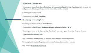
Advantage of CountingSort:
•Counting sort generally performs faster than all comparison-based sorting algorithms, such as merge sort
and quicksort, if the range of input is of the order of the number of input.
•Counting sort is easy to code
•Counting sort is a stable algorithm.
Disadvantage of Counting Sort:
•Counting sort doesn’t work on decimal values.
•Counting sort is inefficient if the range of values to be sorted is very large.
•Counting sort is not an In-place sorting algorithm, It uses extra space for sorting the array elements.
Applications of Counting Sort:
•It is a commonly used algorithm for the cases where we have limited range items.
For example, sort students by grades, sort a events by time, days, months, years, etc.
•It is used in Radix Sort, Bucket Sort .
.
10.
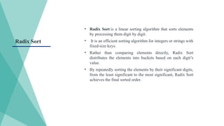
• Radix Sortis a linear sorting algorithm that sorts elements
by processing them digit by digit.
• It is an efficient sorting algorithm for integers or strings with
fixed-size keys.
• Rather than comparing elements directly, Radix Sort
distributes the elements into buckets based on each digit’s
value.
• By repeatedly sorting the elements by their significant digits,
from the least significant to the most significant, Radix Sort
achieves the final sorted order.
Radix Sort
11.
Radix Sort
Algorithm work?
Step1: Find the largest
element in the array, which is
802. It has three digits, so we
will iterate three times, once
for each significant place.
Step 2: Sort the elements based on the unit place digits (X=0).
We use a stable sorting technique, such as counting sort, to
sort the digits at each significant place. It’s important to
understand that the default implementation of counting sort
is unstable i.e. same keys can be in a different order than the
input array. To solve this problem, We can iterate the input
array in reverse order to build the output array. This strategy
helps us to keep the same keys in the same order as they
appear in the input array.
Sorting based on the unit place:
•Perform counting sort on the array based on the unit place
digits.
•The sorted array based on the unit place is [170, 90, 802, 2,
24, 45, 75, 66].
12.
Step 3: Sortthe elements based on the tens place digits.
Sorting based on the tens place:
•Perform counting sort on the array based on the tens
place digits.
•The sorted array based on the tens place is [802, 2, 24,
45, 66, 170, 75, 90].
Step 4: Sort the elements based on the hundreds place
digits.
Sorting based on the hundreds place:
•Perform counting sort on the array based on the
hundreds place digits.
•The sorted array based on the hundreds place is [2, 24,
45, 66, 75, 90, 170, 802].
Step 5: The array is now sorted in ascending order.
The final sorted array using radix sort is [2, 24, 45, 66, 75, 90,
170, 802].
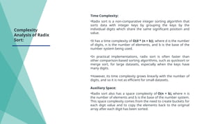
Time Complexity:
•Radix sortis a non-comparative integer sorting algorithm that
sorts data with integer keys by grouping the keys by the
individual digits which share the same significant position and
value.
•It has a time complexity of O(d * (n + b)), where d is the number
of digits, n is the number of elements, and b is the base of the
number system being used.
•In practical implementations, radix sort is often faster than
other comparison-based sorting algorithms, such as quicksort or
merge sort, for large datasets, especially when the keys have
many digits.
•However, its time complexity grows linearly with the number of
digits, and so it is not as efficient for small datasets.
Auxiliary Space:
•Radix sort also has a space complexity of O(n + b), where n is
the number of elements and b is the base of the number system.
This space complexity comes from the need to create buckets for
each digit value and to copy the elements back to the original
array after each digit has been sorted.
Complexity
Analysis of Radix
Sort:
15.
Advantages of RadixSort:
•Radix sort has a, linear time complexity[the runtime of an algorithm
increases in a linear fashion as the size of its input increases] which
makes it faster than comparison-based sorting algorithms such as quicksort and
merge sort for large data sets.
•It is a stable sorting algorithm, meaning that elements with the same key
value maintain their relative order in the sorted output.
•Radix sort is efficient for sorting large numbers of integers or strings.
Disadvantages of Radix Sort:
•Radix sort is not efficient for sorting floating-point numbers or other types
of data that cannot be easily mapped to a small number of digits.
•It requires a significant amount of memory to hold the count of the number
of times each digit value appears.
•It is not efficient for small data sets or data sets with a small number of
unique keys.
Applications of Radix Sort
•In a typical computer, which is a sequential random-access
machine, where the records are keyed by multiple fields radix sort
is used.
For eg., you want to sort on three keys month, day, and year. You
could compare two records on year, then on a tie on month and
finally on the date. Alternatively, sorting the data three times using
Radix sort first on the date, then on month, and finally on year
could be used.
•It was used in card sorting machines with 80 columns, and in each
column, the machine could punch a hole only in 12 places. The
sorter was then programmed to sort the cards, depending upon
which place the card had been punched. This was then used by the
operator to collect the cards which had the 1st row punched,
followed by the 2nd row, and so on.
16.
Lower Bound TheoryConcept is based upon the calculation of minimum time that is
required to execute an algorithm is known as a lower bound theory or Base Bound
Theory.
Concept/Aim: The main aim is to calculate a minimum number of comparisons
required to execute an algorithm.
Lower bound theory-
According to the lower bound theory, for a lower bound (Ln) of an algorithm, it is not
possible to have any algorithm (for a common problem) whose time Complexity is
Less than L(n) for random input.
Once lower bound is calculated, then we can compare it with the actual complexity of
the algorithms & if their Order are same then we con declare our algorithm as optimal.
Lower Bound Theory uses a number of methods/techniques to find out the lower
bound.
Techniques:
1.Comparisons Trees.
2.Oracle and adversary argument
3.Techniques for Algebraic Problem
Lower Bound Theory
17.
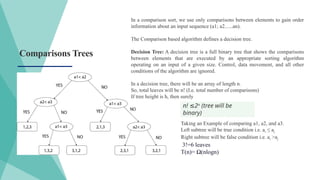
Comparisons Trees
In acomparison sort, we use only comparisons between elements to gain order
information about an input sequence (a1; a2......an).
The Comparison based algorithm defines a decision tree.
Decision Tree: A decision tree is a full binary tree that shows the comparisons
between elements that are executed by an appropriate sorting algorithm
operating on an input of a given size. Control, data movement, and all other
conditions of the algorithm are ignored.
In a decision tree, there will be an array of length n.
So, total leaves will be n! (I.e. total number of comparisons)
If tree height is h, then surely
n! 2
≤ n
(tree will be
binary)
Taking an Example of comparing a1, a2, and a3.
Left subtree will be true condition i.e. ai ≤ aj
Right subtree will be false condition i.e. ai >aj
3!=6 leaves
T(n)= Ω(nlogn)
18.
Oracle and adversary
argument:
•Another technique for obtaining lower bounds consists of making use of an "oracle.“
• Oracle use Decicion Tree to find out Lower bound.
19.
Using Lower bondtheory to solve the algebraic problem:
1. Straight Line Program –
The type of program built without any loops or control structures is called the Straight-Line Program.
• For example, Sum of Two numbers
Sum(int a, int b)
{
int c = a + b;
return c;
}
2. Algebraic Problem –
Problems related to algebra like solving equations inequalities etc. come under algebraic problems.
• For example, solving equation ax2
+bx+c with simple programming.
=> an
xn
+an-1
xn-1
+an-2
xn-2
+...+a1
x+a0 polynomial(A, x, n)
{ int p, v=0; // loop executed n times
for i = 0 to n
v = (v + A[i])*x;
return v;
}
20.
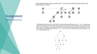
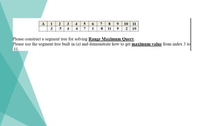
1. Sort thefollowing list using the Radix sort algorithm.
329, 457, 839, 436, 720, 355, 657
2. Consider the following unsorted array:
a[] = {19, 2, 18, 400, 67, 234, 649, 128}
3. Sort the following list using the Counting sort algorithm.
4. We have a list of items according to the following Position:
1,2,3,4,5,6,7,8,9,10,11,12,13,14
Find out lower bound .
Assignment
21.
A fibonacci heapis a data structure that consists of a collection of trees
which follow min heap or max heap property.
1.A min-heap is a tree in which, for all the nodes, the key value of the
parent must be smaller than the key value of the children.
2.A max-heap is a tree in which, for all the nodes, the key value of the
parent must be greater than the key value of the children.
These two properties are the characteristics of the
trees present on a fibonacci heap.
Fibonacci Heaps
In a fibonacci heap, a node can have more than two children or no children at all.
It is not restricted to a binary tree structure (where each node can have at most 2 children). Instead, a node in a
Fibonacci Heap can have any number of children (0, 1, 2, 3, 4, etc.), depending on how the heap operations have
been performed.
The fibonacci heap is called a fibonacci heap because the trees are constructed in a way such that a tree of order n has at
least Fn+2
nodes in it, where Fn+2
is the (n + 2)th
Fibonacci number.
22.
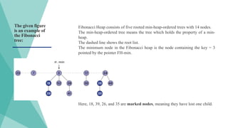
The given figure
isan example of
the Fibonacci
tree:
Fibonacci Heap consists of five rooted min-heap-ordered trees with 14 nodes.
The min-heap-ordered tree means the tree which holds the property of a min-
heap.
The dashed line shows the root list.
The minimum node in the Fibonacci heap is the node containing the key = 3
pointed by the pointer FH-min.
Here, 18, 39, 26, and 35 are marked nodes, meaning they have lost one child.
23.
Properties of aFibonacci Heap
Important properties of a Fibonacci heap are:
1.It is a set of min heap-ordered trees. (i.e. The parent is always smaller
than the children.)
2.A pointer is maintained at the minimum element node.
3.It consists of a set of marked nodes. (Decrease key operation)
4.The trees within a Fibonacci heap are unordered but rooted.
24.
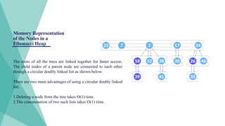
Memory Representation
of theNodes in a
Fibonacci Heap
The roots of all the trees are linked together for faster access.
The child nodes of a parent node are connected to each other
through a circular doubly linked list as shown below.
There are two main advantages of using a circular doubly linked
list.
1.Deleting a node from the tree takes O(1) time.
2.The concatenation of two such lists takes O(1) time.
25.
Insertion of anode: insert(H, x)
degree[x] = 0
p[x] = NIL
child[x] = NIL
left[x] = x
right[x] = x
mark[x] = FALSE
concatenate the root list containing x with root list H
if min[H] == NIL or key[x] < key[min[H]]
then min[H] = x
n[H] = n[H] + 1
Inserting a node into an already existing heap follows the
steps below.
1.Create a new node for the element.
2.Check if the heap is empty.
3.If the heap is empty, set the new node as a root node and
mark it min.
4.Else, insert the node into the root list and update min.
Union of two
FibonacciHeap:
UNION-FIB-HEAP (FH1, FH2)
1. FH = MAKE-FIB-HEAP ()
2. FH -> min = FH1 -> Min
3. Concatenating the root list of FH2 with the root list of FH
4. If (FH1 -> == Nil) or (H2 -> min != NIL and FH2 -> min -
> key < H1 -> min -> key)
5. FH - > min = FH2 -> min
6. FH -> n = FH1 -> n + FH2 -> n
7. Return FH
Union of two fibonacci heaps consists of following steps.
1.Concatenate the roots of both the heaps.
2.Update min by selecting a minimum key from the new root lists.
28.
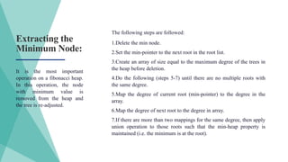
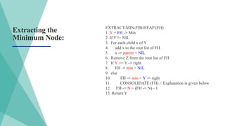
Extracting the
Minimum Node:
Thefollowing steps are followed:
1.Delete the min node.
2.Set the min-pointer to the next root in the root list.
3.Create an array of size equal to the maximum degree of the trees in
the heap before deletion.
4.Do the following (steps 5-7) until there are no multiple roots with
the same degree.
5.Map the degree of current root (min-pointer) to the degree in the
array.
6.Map the degree of next root to the degree in array.
7.If there are more than two mappings for the same degree, then apply
union operation to those roots such that the min-heap property is
maintained (i.e. the minimum is at the root).
It is the most important
operation on a fibonacci heap.
In this operation, the node
with minimum value is
removed from the heap and
the tree is re-adjusted.
29.
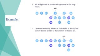
Example:
1. We willperform an extract-min operation on the heap
below.
2. Delete the min node, add all its child nodes to the root list
and set the min-pointer to the next root in the root list..
30.
Example:
3. The maximumdegree in the tree is 3. Create an array of size 4 and map degree of
the next roots with the array.
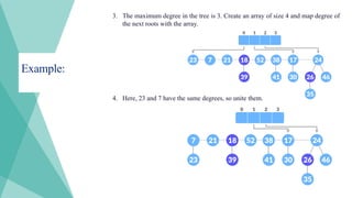
4. Here, 23 and 7 have the same degrees, so unite them.
31.
Example:
5. Again, 7and 17 have the same degrees, so unite them as well.
6. Again 7 and 24 have the same degree, so unite them.
32.
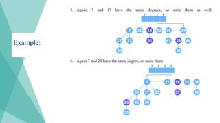
Example:
7. Map thenext nodes.
8. Again, 52 and 21 have the same degree, so unite them.
Extracting the
Minimum Node:
EXTRACT-MIN-FIB-HEAP(FH)
1. Y = FH -> Min
2. If Y != NIL
3. For each child x of Y
4. add x to the root list of FH
5. x -> parent = NIL
6. Remove Z from the root list of FH
7. If Y == Y -> right
8. FH -> min = NIL
9. else
10. FH -> min = Y -> right
11. CONSOLIDATE (FH) // Explanation is given below
12. FH -> N = (FH -> N) - 1
13. Return Y
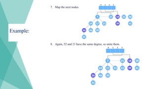
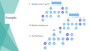
35.
Decreasing a
Key
To decreasethe value of any element in the heap, we follow the following algorithm:
•Decrease the value of the node ‘x’ to the new chosen value.
•CASE 1) If min-heap property is not violated,
• Update min pointer if necessary.
•CASE 2) If min-heap property is violated and parent of ‘x’ is unmarked,
• Cut off the link between ‘x’ and its parent.
• Mark the parent of ‘x’.
• Add tree rooted at ‘x’ to the root list and update min pointer if necessary.
•CASE 3)If min-heap property is violated and parent of ‘x’ is marked,
• Cut off the link between ‘x’ and its parent p[x].
• Add ‘x’ to the root list, updating min pointer if necessary.
• Cut off link between p[x] and p[p[x]].
• Add p[x] to the root list, updating min pointer if necessary.
• If p[p[x]] is unmarked, mark it.
• Else, cut off p[p[x]] and repeat steps , taking p[p[x]] as ‘x’.
36.
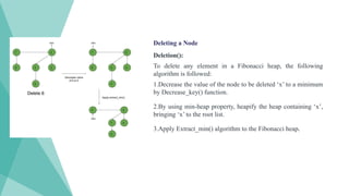
Deletion():
To delete anyelement in a Fibonacci heap, the following
algorithm is followed:
1.Decrease the value of the node to be deleted ‘x’ to a minimum
by Decrease_key() function.
2.By using min-heap property, heapify the heap containing ‘x’,
bringing ‘x’ to the root list.
3.Apply Extract_min() algorithm to the Fibonacci heap.
Deleting a Node
Red-Black Tree
• ARed-Black Tree is a self-balancing binary search tree
where each node has an additional attribute:
a color, which can be either red or black.
• The primary objective of these trees is to
maintain balance during insertions and deletions,
ensuring efficient data retrieval and manipulation.
39.
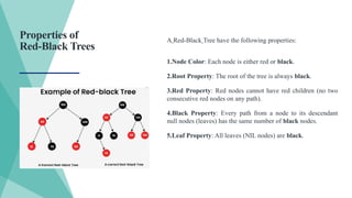
Properties of
Red-Black Trees
ARed-Black Tree have the following properties:
1.Node Color: Each node is either red or black.
2.Root Property: The root of the tree is always black.
3.Red Property: Red nodes cannot have red children (no two
consecutive red nodes on any path).
4.Black Property: Every path from a node to its descendant
null nodes (leaves) has the same number of black nodes.
5.Leaf Property: All leaves (NIL nodes) are black.
40.
Basic Operations onRed-Black Tree
The basic operations on a Red-Black Tree include:
1. Insertion
2. Search
3. Deletion
41.
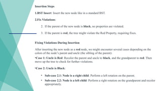
Insertion Steps
1.BST Insert:Insert the new node like in a standard BST.
2.Fix Violations:
2. If the parent of the new node is black, no properties are violated.
3. If the parent is red, the tree might violate the Red Property, requiring fixes.
Fixing Violations During Insertion
After inserting the new node as a red node, we might encounter several cases depending on the
colors of the node’s parent and uncle (the sibling of the parent):
•Case 1: Uncle is Red: Recolor the parent and uncle to black, and the grandparent to red. Then
move up the tree to check for further violations.
•Case 2: Uncle is Black:
• Sub-case 2.1: Node is a right child: Perform a left rotation on the parent.
• Sub-case 2.2: Node is a left child: Perform a right rotation on the grandparent and recolor
appropriately.
42.
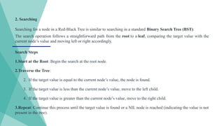
2. Searching
Searching fora node in a Red-Black Tree is similar to searching in a standard Binary Search Tree (BST).
The search operation follows a straightforward path from the root to a leaf, comparing the target value with the
current node’s value and moving left or right accordingly.
Search Steps
1.Start at the Root: Begin the search at the root node.
2.Traverse the Tree:
2. If the target value is equal to the current node’s value, the node is found.
3. If the target value is less than the current node’s value, move to the left child.
4. If the target value is greater than the current node’s value, move to the right child.
3.Repeat: Continue this process until the target value is found or a NIL node is reached (indicating the value is not
present in the tree).
43.
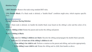
Deletion Steps
1.BST Deletion:Remove the node using standard BST rules.
2.Fix Double Black: If a black node is deleted, a “double black” condition might arise, which requires specific
fixes.
Fixing Violations During Deletion
When a black node is deleted, we handle the double black issue based on the sibling’s color and the colors of its
children:
•Case 1: Sibling is Red: Rotate the parent and recolor the sibling and parent.
•Case 2: Sibling is Black:
• Sub-case 2.1: Sibling’s children are black: Recolor the sibling and propagate the double black upwards.
• Sub-case 2.2: At least one of the sibling’s children is red:
• If the sibling’s far child is red: Perform a rotation on the parent and sibling, and recolor appropriately.
• If the sibling’s near child is red: Rotate the sibling and its child, then handle as above.
44.
Find out
Advantages andDisadvantages of Red-Black Trees
Applications of Red-Black Trees
Time Complexity of Red-Black Trees
45.
A Segment Treeis used to stores information about array intervals in its nodes.
•It allows efficient range queries over array intervals.
•Along with queries, it allows efficient updates of array items.
•For example, we can perform a range summation of an array between the range L to R in O(Log n) while
also modifying any array element in O(Log n) Time
Segment Trees
46.
Segment Trees aremainly used for range queries on a fixed sized array.
The values of array elements can be changed.
Example queries over a range in an array.
•Addition/Subtraction
•Maximum/Minimum
Types of Operations in
Segment Trees
47.
Structure of theTree
The segment tree works on the principle of divide and conquer.
•At each level, we divide the array segments into two parts. If the given array had [0, . . ., N-1] elements in it
then the two parts of the array will be [0, . . ., N/2-1] and [N/2, . . ., N-1].
•The structure of the segment tree looks like a binary tree.
48.
Constructing the segmenttree
There are two important points :
•Choosing what value to be stored in the nodes according to the problem definition
•What should the merge operation do
If the problem definition states that we need to calculate the sum over ranges, then the value at nodes
should store the sum of values over the ranges.
•The child node values are merged back into the parent node to hold the value for that particular range,
[i.e., the range covered by all the nodes of its subtree].
•In the end, leaf nodes store information about a single element. All the leaf nodes store the array based
on which the segment tree is built.
49.
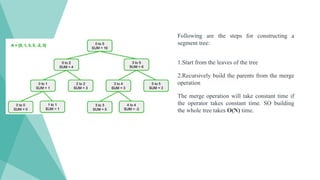
Following are thesteps for constructing a
segment tree:
1.Start from the leaves of the tree
2.Recursively build the parents from the merge
operation
The merge operation will take constant time if
the operator takes constant time. SO building
the whole tree takes O(N) time.
50.
Range Query
The firststep is constructing the segment tree with
the addition operator and 0 as the neutral element.
•If the range is one of the node’s range values then
simply return the answer.
•Otherwise, we will need to traverse the left and right
children of the nodes and recursively continue the
process till we find a node that covers a range that
totally covers a part or whole of the range [L, R]
•While returning from each call, we need to merge
the answers received from each of its child.
As the height of the segment tree is logN the query
time will be O(logN) per query.
51.
Point Updates
Given anindex, idx, update the value of the array at index idx with value V
The element’s contribution is only in the path from
its leaf to its parent. Thus only logN elements will
get affected due to the update.
For updating, traverse till the leaf that stores the
value of index idx and update the value. Then while
tracing back in the path, modify the ranges
accordingly.
The time complexity will be O(logN).
52.
What are theapplications, advantages and disadvantages of
Segment trees?
53.
Fenwick Tree
Binary IndexedTree also called Fenwick Tree provides a way to represent an array of numbers in
an array, allowing prefix sums to be calculated efficiently.
For example, an array is [2, 3, -1, 0, 6] the length 3 prefix [2, 3, -1] with sum 2 + 3 + -1 = 4).
Calculating a prefix sum takes time based on the size of the array. If you have to do this many
times in a mixed set of operations, it will take too long and might not finish in a reasonable time.
Using binary Indexed tree also, we can perform both the tasks in O(logN) time.
54.
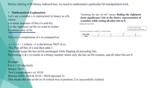
Before starting withbinary indexed tree, we need to understand a particular bit manipulation trick.
"Isolating the last set bit" means finding the rightmost
(least significant) 1-bit in the binary representation of
a number while setting all other bits to 0.
• Mathematical Explanation
Let’s say a number x is represented in binary as a1b,
where:
a is some sequence of bits (1s and 0s).
1 is the rightmost set bit we want to isolate.
b consists only of 0s.
The two’s complement of x is computed as:
-x = (~x) + 1 (where ~x is the bitwise NOT of x).
This flips all bits of x and then adds 1.
The result keeps the last set bit unchanged while flipping all preceding bits.
Performing x & (-x) results in a binary number where only the last set bit remains, and all other bits are 0.
Example
For x = 10 (decimal):
Binary: 1010
Two’s complement (-x): 0110
Bitwise AND: 1010 & 0110 = 0010 (decimal 2)
This means the last set bit in 10 (which was at position 2) is successfully isolated.
55.
Basic Idea
We usethe fact that any integer can be represented as a sum of powers
of 2.
How does BIT work?
•Instead of storing individual elements, BIT stores partial sums at each
index.
•Each index in BIT covers a specific range of elements from the original
array, determined by its last set bit.
•We can efficiently update and retrieve prefix sums using bit
manipulation.
•Example : int a[] = {0, 1, 2, 3, 4, 5, 6, 7, 8, 9, 10, 11, 12, 13, 14, 15, 16};
•Each BIT[i] stores the sum of elements from i - (1 << r) + 1 to i, where r
is the last set bit in i.
56.
Sum of first12 numbers in array a[] = BIT[12] + BIT[8] = (a[12] + … + a[9]) + (a[8] + … + a[1])
Similarly, sum of first 6 elements = BIT[6] + BIT[4] = (a[6] + a[5]) + (a[4] + … + a[1])
Sum of first 8 elements = BIT[8] = a[8] + … + a[1]
Let’s see how to construct this tree .
BIT[] is an array of size = 1 + the size of the given array a[]
on which we need to perform operations.
Initially all values in BIT[] are equal to 0.
Then we call update() operation for each element of given
array to construct the Binary Indexed Tree.
The update() operation is discussed below.
Example of update(13, 2)
We update a[13] by adding 2, and then propagate this change to other relevant BIT indices.
Steps:
x = 13 (1101 in binary)
Update BIT[13] += 2
Find last set bit: 13 & -13 = 1
Move to x = 13 + 1 = 14
x = 14 (1110 in binary)
The indices 13, 14, 16 cover index 13, so they all need to be updated.
The update propagates upwards using bit manipulation.
Update BIT[14] += 2
Find last set bit: 14 & -14 = 2
Move to x = 14 + 2 = 16
x = 16 (10000 in binary)
Update BIT[16] += 2
Find last set bit: 16 & -16 = 16
Move to x = 16 + 16 = 32 (out of bounds, stop)
57.
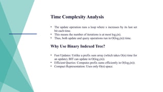
Time Complexity Analysis
•The update operation runs a loop where x increases by its last set
bit each time.
• This means the number of iterations is at most log (n).
₂
• Thus, both update and query operations run in O(log (n)) time.
₂
Why Use Binary Indexed Tree?
• Fast Updates: Unlike a prefix sum array (which takes O(n) time for
an update), BIT can update in O(log (n)).
₂
• Efficient Queries: Computes prefix sums efficiently in O(log (n)).
₂
• Compact Representation: Uses only O(n) space.

![Counting Sort
• Counting Sort is a non-comparison-based sorting
algorithm. [ used to arrange data without comparing
elements directly.]
• It is particularly efficient when the range of input values is
small compared to the number of elements to be sorted.
• The basic idea behind Counting Sort is to count
the frequency of each distinct element in the input array and
use that information to place the elements in their correct
sorted positions.
• For example, for input [1, 4, 3, 2, 2, 1], the output should be
[1, 1, 2, 2, 3, 4].](https://image.slidesharecdn.com/aa2-250804083515-7d4cbd73/85/Advance-Algorithm_unit_2_czcbcnhgjy-pptx-2-320.jpg)
![Working of
Counting Sort
Find out the maximum element
from the given array.
Initialize a countArray[] of
length max+1 with all elements as 0.
This array will be used for storing the occurrences
of the elements of the input array.
countArray[], store the count of each unique
element of the input array at their respective
indices.
Store the cumulative sum or prefix sum of the
elements of the countArray[] by doing
countArray[i] = countArray[i – 1] +
countArray[i].
This will help in placing the elements of the input
array at the correct index in the output array.](https://image.slidesharecdn.com/aa2-250804083515-7d4cbd73/85/Advance-Algorithm_unit_2_czcbcnhgjy-pptx-3-320.jpg)
![•Update outputArray[ countArray[ inputArray[i] ] – 1] = inputArray[i].
•Also, update countArray[ inputArray[i] ] = countArray[ inputArray[i] ].
For i = 6,
Update outputArray[ countArray[ inputArray[6] ] – 1] = inputArray[6]
Also, update countArray[ inputArray[6] ] = countArray[ inputArray[6] ]
For i = 5,
Update outputArray[ countArray[ inputArray[5] ] – 1] = inputArray[5]
Also, update countArray[ inputArray[5] ] = countArray[ inputArray[5] ]
For i = 4,
Update outputArray[ countArray[ inputArray[4] ] – 1] = inputArray[4]
Also, update countArray[ inputArray[4] ] = countArray[ inputArray[4] ]](https://image.slidesharecdn.com/aa2-250804083515-7d4cbd73/85/Advance-Algorithm_unit_2_czcbcnhgjy-pptx-4-320.jpg)
![For i = 3,
Update outputArray[ countArray[ inputArray[3] ] – 1] = inputArray[3]
Also, update countArray[ inputArray[3] ] = countArray[ inputArray[3] ]
For i = 2,
Update outputArray[ countArray[ inputArray[2] ] – 1] = inputArray[2]
Also, update countArray[ inputArray[2] ] = countArray[ inputArray[2] ]
For i = 1,
Update outputArray[ countArray[ inputArray[1] ] – 1] = inputArray[1]
Also, update countArray[ inputArray[1] ] = countArray[ inputArray[1] ]
For i = 0,
Update outputArray[ countArray[ inputArray[0] ] – 1] = inputArray[0]
Also, update countArray[ inputArray[0] ] = countArray[ inputArray[0] ]](https://image.slidesharecdn.com/aa2-250804083515-7d4cbd73/85/Advance-Algorithm_unit_2_czcbcnhgjy-pptx-5-320.jpg)
![Counting Sort
1. [11,11,7,9,9,12,11,10,11,9,12,7,11,9,7,8,11,11,6,10]](https://image.slidesharecdn.com/aa2-250804083515-7d4cbd73/85/Advance-Algorithm_unit_2_czcbcnhgjy-pptx-6-320.jpg)
![Counting Sort
Algorithm:
•Declare an auxiliary array countArray[] of size max(inputArray[])+1 and
initialize it with 0.
•Traverse array inputArray[] and map each element of inputArray[] as an
index of countArray[] array, i.e., execute countArray[inputArray[i]]+
+ for 0 <= i < N.
•Calculate the prefix sum at every index of array inputArray[].
•Create an array outputArray[] of size N.
•Traverse array inputArray[] from end and
update outputArray[ countArray[ inputArray[i] ] – 1] = inputArray[i].
•Also, update countArray[ inputArray[i] ] = countArray[ inputArray[i] ]
.](https://image.slidesharecdn.com/aa2-250804083515-7d4cbd73/85/Advance-Algorithm_unit_2_czcbcnhgjy-pptx-7-320.jpg)
![Complexity Analysis of Counting Sort:
•Time Complexity: O(N+M), where N and M are the size
of inputArray[] and countArray[] respectively.
• Worst-case: O(N+M).
• Average-case: O(N+M).
• Best-case: O(N+M).
•Auxiliary Space: O(N+M), where N and M are the space taken
by outputArray[] and countArray[] respectively](https://image.slidesharecdn.com/aa2-250804083515-7d4cbd73/85/Advance-Algorithm_unit_2_czcbcnhgjy-pptx-8-320.jpg)
![Radix Sort
Algorithm work?
Step 1: Find the largest
element in the array, which is
802. It has three digits, so we
will iterate three times, once
for each significant place.
Step 2: Sort the elements based on the unit place digits (X=0).
We use a stable sorting technique, such as counting sort, to
sort the digits at each significant place. It’s important to
understand that the default implementation of counting sort
is unstable i.e. same keys can be in a different order than the
input array. To solve this problem, We can iterate the input
array in reverse order to build the output array. This strategy
helps us to keep the same keys in the same order as they
appear in the input array.
Sorting based on the unit place:
•Perform counting sort on the array based on the unit place
digits.
•The sorted array based on the unit place is [170, 90, 802, 2,
24, 45, 75, 66].](https://image.slidesharecdn.com/aa2-250804083515-7d4cbd73/85/Advance-Algorithm_unit_2_czcbcnhgjy-pptx-11-320.jpg)
![Step 3: Sort the elements based on the tens place digits.
Sorting based on the tens place:
•Perform counting sort on the array based on the tens
place digits.
•The sorted array based on the tens place is [802, 2, 24,
45, 66, 170, 75, 90].
Step 4: Sort the elements based on the hundreds place
digits.
Sorting based on the hundreds place:
•Perform counting sort on the array based on the
hundreds place digits.
•The sorted array based on the hundreds place is [2, 24,
45, 66, 75, 90, 170, 802].
Step 5: The array is now sorted in ascending order.
The final sorted array using radix sort is [2, 24, 45, 66, 75, 90,
170, 802].](https://image.slidesharecdn.com/aa2-250804083515-7d4cbd73/85/Advance-Algorithm_unit_2_czcbcnhgjy-pptx-12-320.jpg)
![Radix Sort
1. Given array [121, 432, 564, 23, 1, 45, 788], sort this array using Radix sort.
2. [127,324,173,4,38,217,134] Sort array.](https://image.slidesharecdn.com/aa2-250804083515-7d4cbd73/85/Advance-Algorithm_unit_2_czcbcnhgjy-pptx-13-320.jpg)
![Advantages of Radix Sort:
•Radix sort has a, linear time complexity[the runtime of an algorithm
increases in a linear fashion as the size of its input increases] which
makes it faster than comparison-based sorting algorithms such as quicksort and
merge sort for large data sets.
•It is a stable sorting algorithm, meaning that elements with the same key
value maintain their relative order in the sorted output.
•Radix sort is efficient for sorting large numbers of integers or strings.
Disadvantages of Radix Sort:
•Radix sort is not efficient for sorting floating-point numbers or other types
of data that cannot be easily mapped to a small number of digits.
•It requires a significant amount of memory to hold the count of the number
of times each digit value appears.
•It is not efficient for small data sets or data sets with a small number of
unique keys.
Applications of Radix Sort
•In a typical computer, which is a sequential random-access
machine, where the records are keyed by multiple fields radix sort
is used.
For eg., you want to sort on three keys month, day, and year. You
could compare two records on year, then on a tie on month and
finally on the date. Alternatively, sorting the data three times using
Radix sort first on the date, then on month, and finally on year
could be used.
•It was used in card sorting machines with 80 columns, and in each
column, the machine could punch a hole only in 12 places. The
sorter was then programmed to sort the cards, depending upon
which place the card had been punched. This was then used by the
operator to collect the cards which had the 1st row punched,
followed by the 2nd row, and so on.](https://image.slidesharecdn.com/aa2-250804083515-7d4cbd73/85/Advance-Algorithm_unit_2_czcbcnhgjy-pptx-15-320.jpg)


![Using Lower bond theory to solve the algebraic problem:
1. Straight Line Program –
The type of program built without any loops or control structures is called the Straight-Line Program.
• For example, Sum of Two numbers
Sum(int a, int b)
{
int c = a + b;
return c;
}
2. Algebraic Problem –
Problems related to algebra like solving equations inequalities etc. come under algebraic problems.
• For example, solving equation ax2
+bx+c with simple programming.
=> an
xn
+an-1
xn-1
+an-2
xn-2
+...+a1
x+a0 polynomial(A, x, n)
{ int p, v=0; // loop executed n times
for i = 0 to n
v = (v + A[i])*x;
return v;
}](https://image.slidesharecdn.com/aa2-250804083515-7d4cbd73/85/Advance-Algorithm_unit_2_czcbcnhgjy-pptx-19-320.jpg)
![1. Sort the following list using the Radix sort algorithm.
329, 457, 839, 436, 720, 355, 657
2. Consider the following unsorted array:
a[] = {19, 2, 18, 400, 67, 234, 649, 128}
3. Sort the following list using the Counting sort algorithm.
4. We have a list of items according to the following Position:
1,2,3,4,5,6,7,8,9,10,11,12,13,14
Find out lower bound .
Assignment](https://image.slidesharecdn.com/aa2-250804083515-7d4cbd73/85/Advance-Algorithm_unit_2_czcbcnhgjy-pptx-20-320.jpg)


![Insertion of a node: insert(H, x)
degree[x] = 0
p[x] = NIL
child[x] = NIL
left[x] = x
right[x] = x
mark[x] = FALSE
concatenate the root list containing x with root list H
if min[H] == NIL or key[x] < key[min[H]]
then min[H] = x
n[H] = n[H] + 1
Inserting a node into an already existing heap follows the
steps below.
1.Create a new node for the element.
2.Check if the heap is empty.
3.If the heap is empty, set the new node as a root node and
mark it min.
4.Else, insert the node into the root list and update min.](https://image.slidesharecdn.com/aa2-250804083515-7d4cbd73/85/Advance-Algorithm_unit_2_czcbcnhgjy-pptx-25-320.jpg)


![Decreasing a
Key
To decrease the value of any element in the heap, we follow the following algorithm:
•Decrease the value of the node ‘x’ to the new chosen value.
•CASE 1) If min-heap property is not violated,
• Update min pointer if necessary.
•CASE 2) If min-heap property is violated and parent of ‘x’ is unmarked,
• Cut off the link between ‘x’ and its parent.
• Mark the parent of ‘x’.
• Add tree rooted at ‘x’ to the root list and update min pointer if necessary.
•CASE 3)If min-heap property is violated and parent of ‘x’ is marked,
• Cut off the link between ‘x’ and its parent p[x].
• Add ‘x’ to the root list, updating min pointer if necessary.
• Cut off link between p[x] and p[p[x]].
• Add p[x] to the root list, updating min pointer if necessary.
• If p[p[x]] is unmarked, mark it.
• Else, cut off p[p[x]] and repeat steps , taking p[p[x]] as ‘x’.](https://image.slidesharecdn.com/aa2-250804083515-7d4cbd73/85/Advance-Algorithm_unit_2_czcbcnhgjy-pptx-35-320.jpg)


![Structure of the Tree
The segment tree works on the principle of divide and conquer.
•At each level, we divide the array segments into two parts. If the given array had [0, . . ., N-1] elements in it
then the two parts of the array will be [0, . . ., N/2-1] and [N/2, . . ., N-1].
•The structure of the segment tree looks like a binary tree.](https://image.slidesharecdn.com/aa2-250804083515-7d4cbd73/85/Advance-Algorithm_unit_2_czcbcnhgjy-pptx-47-320.jpg)
![Constructing the segment tree
There are two important points :
•Choosing what value to be stored in the nodes according to the problem definition
•What should the merge operation do
If the problem definition states that we need to calculate the sum over ranges, then the value at nodes
should store the sum of values over the ranges.
•The child node values are merged back into the parent node to hold the value for that particular range,
[i.e., the range covered by all the nodes of its subtree].
•In the end, leaf nodes store information about a single element. All the leaf nodes store the array based
on which the segment tree is built.](https://image.slidesharecdn.com/aa2-250804083515-7d4cbd73/85/Advance-Algorithm_unit_2_czcbcnhgjy-pptx-48-320.jpg)
![Range Query
The first step is constructing the segment tree with
the addition operator and 0 as the neutral element.
•If the range is one of the node’s range values then
simply return the answer.
•Otherwise, we will need to traverse the left and right
children of the nodes and recursively continue the
process till we find a node that covers a range that
totally covers a part or whole of the range [L, R]
•While returning from each call, we need to merge
the answers received from each of its child.
As the height of the segment tree is logN the query
time will be O(logN) per query.](https://image.slidesharecdn.com/aa2-250804083515-7d4cbd73/85/Advance-Algorithm_unit_2_czcbcnhgjy-pptx-50-320.jpg)


![Fenwick Tree
Binary Indexed Tree also called Fenwick Tree provides a way to represent an array of numbers in
an array, allowing prefix sums to be calculated efficiently.
For example, an array is [2, 3, -1, 0, 6] the length 3 prefix [2, 3, -1] with sum 2 + 3 + -1 = 4).
Calculating a prefix sum takes time based on the size of the array. If you have to do this many
times in a mixed set of operations, it will take too long and might not finish in a reasonable time.
Using binary Indexed tree also, we can perform both the tasks in O(logN) time.](https://image.slidesharecdn.com/aa2-250804083515-7d4cbd73/85/Advance-Algorithm_unit_2_czcbcnhgjy-pptx-53-320.jpg)
![Basic Idea
We use the fact that any integer can be represented as a sum of powers
of 2.
How does BIT work?
•Instead of storing individual elements, BIT stores partial sums at each
index.
•Each index in BIT covers a specific range of elements from the original
array, determined by its last set bit.
•We can efficiently update and retrieve prefix sums using bit
manipulation.
•Example : int a[] = {0, 1, 2, 3, 4, 5, 6, 7, 8, 9, 10, 11, 12, 13, 14, 15, 16};
•Each BIT[i] stores the sum of elements from i - (1 << r) + 1 to i, where r
is the last set bit in i.](https://image.slidesharecdn.com/aa2-250804083515-7d4cbd73/85/Advance-Algorithm_unit_2_czcbcnhgjy-pptx-55-320.jpg)
![Sum of first 12 numbers in array a[] = BIT[12] + BIT[8] = (a[12] + … + a[9]) + (a[8] + … + a[1])
Similarly, sum of first 6 elements = BIT[6] + BIT[4] = (a[6] + a[5]) + (a[4] + … + a[1])
Sum of first 8 elements = BIT[8] = a[8] + … + a[1]
Let’s see how to construct this tree .
BIT[] is an array of size = 1 + the size of the given array a[]
on which we need to perform operations.
Initially all values in BIT[] are equal to 0.
Then we call update() operation for each element of given
array to construct the Binary Indexed Tree.
The update() operation is discussed below.
Example of update(13, 2)
We update a[13] by adding 2, and then propagate this change to other relevant BIT indices.
Steps:
x = 13 (1101 in binary)
Update BIT[13] += 2
Find last set bit: 13 & -13 = 1
Move to x = 13 + 1 = 14
x = 14 (1110 in binary)
The indices 13, 14, 16 cover index 13, so they all need to be updated.
The update propagates upwards using bit manipulation.
Update BIT[14] += 2
Find last set bit: 14 & -14 = 2
Move to x = 14 + 2 = 16
x = 16 (10000 in binary)
Update BIT[16] += 2
Find last set bit: 16 & -16 = 16
Move to x = 16 + 16 = 32 (out of bounds, stop)](https://image.slidesharecdn.com/aa2-250804083515-7d4cbd73/85/Advance-Algorithm_unit_2_czcbcnhgjy-pptx-56-320.jpg)