Downloaded 39 times
![4
• In linear search, access each element of an array one by one sequentially and see whether it
is desired element or not. A search will be unsuccessful if all the elements are accessed and
the desired element is not found.
• In brief, Simply search for the given element left to right and return the index of the
element, if found. Otherwise return “Not Found”.
Algorithm:
LinearSearch(A, n,key)
{
for(i=0;i<n;i++)
{
if(A[i] == key)
return i;
}
return -1; //-1 indicates unsuccessful search
}
Analysis: Time complexity = O(n)
Linear Search](https://image.slidesharecdn.com/unit-8searchingandhashing-171201035421/75/Unit-8-searching-and-hashing-4-2048.jpg)
![6
Iterative Algorithm
BinarySearch(A, l, r, key)
{
while(l<=r)
{
m = (l + r) /2 ; //integer division
if(key = = A[m]
print " Search successful"
else if (key < A[m])
r = m - 1
else
l = m+1
}
If(l>r)
print "unsuccessful search"
}](https://image.slidesharecdn.com/unit-8searchingandhashing-171201035421/75/Unit-8-searching-and-hashing-6-2048.jpg)
![7
BinarySearch(A, l, r, key)
{
if(l= = r) //only one element
{
if(key = = A[l])
print " successful Search"
else
print "unsuccessful Search"
}
else
{
m = (l + r) /2 ; //integer division
if(key = = A[m]
print "successful search"
else if (key < A[m])
return BinarySearch(A, l, m-1, key) ;
else
return BinarySearch(A, m+1, r, key) ;
}
}
Algorithm: Recursive](https://image.slidesharecdn.com/unit-8searchingandhashing-171201035421/75/Unit-8-searching-and-hashing-7-2048.jpg)
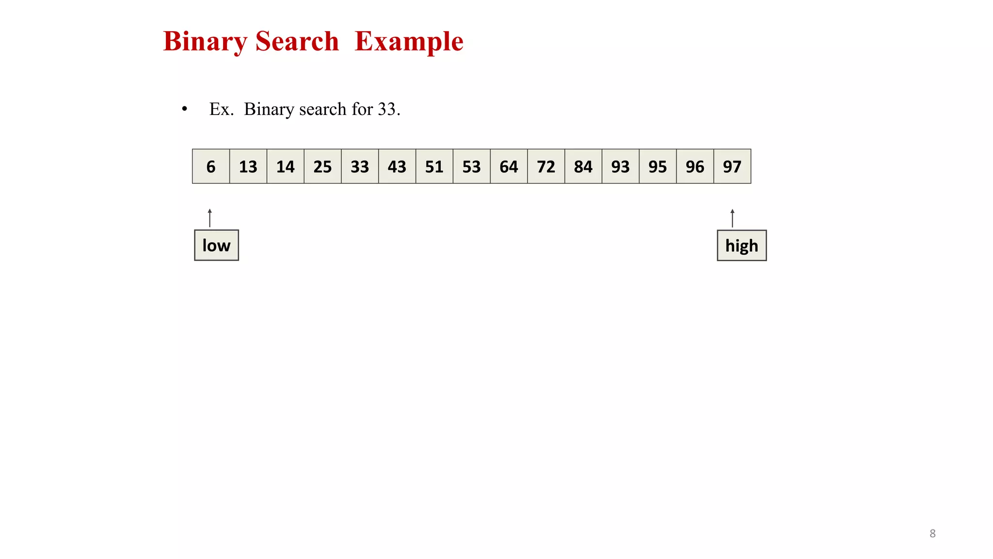
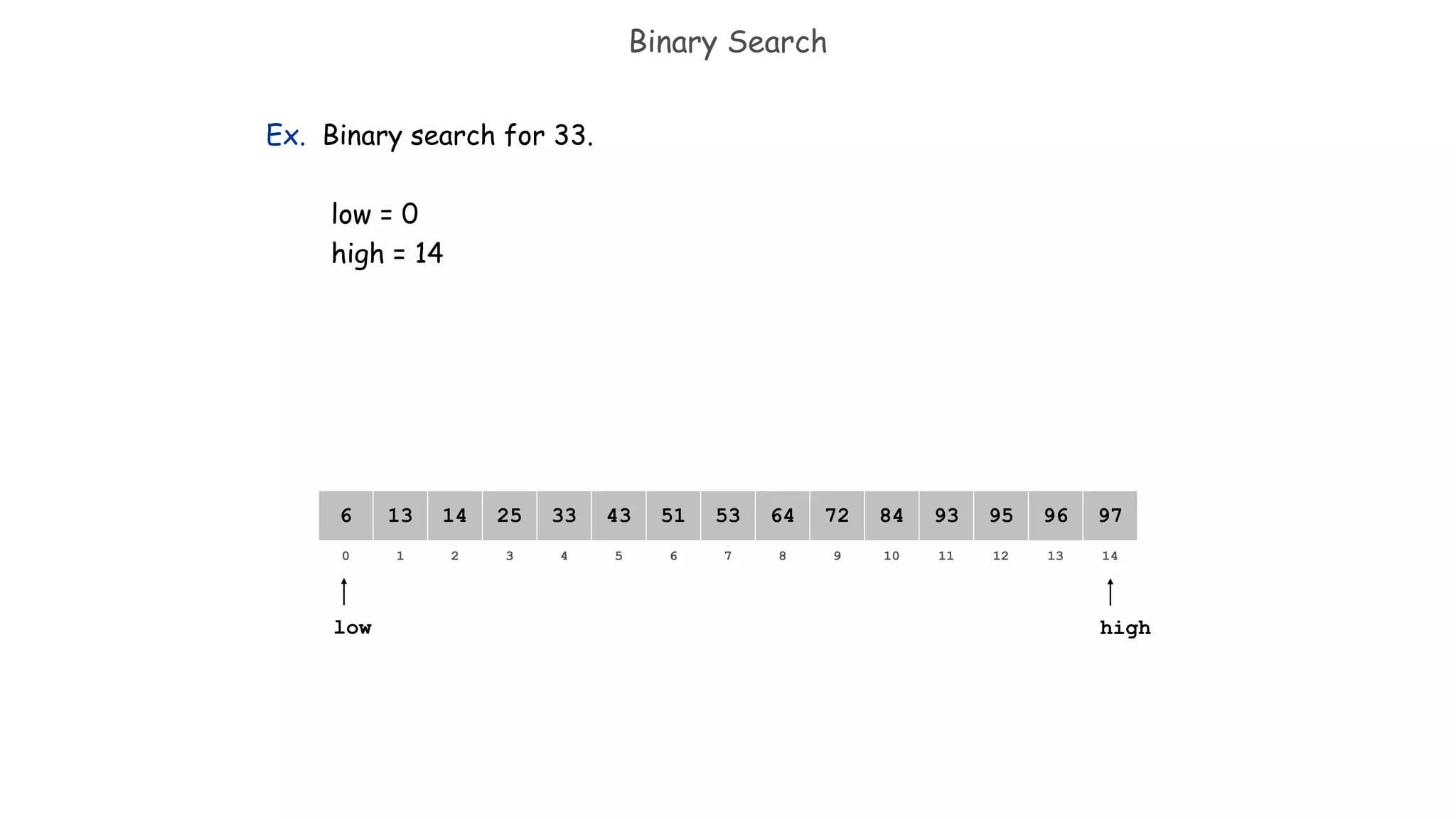
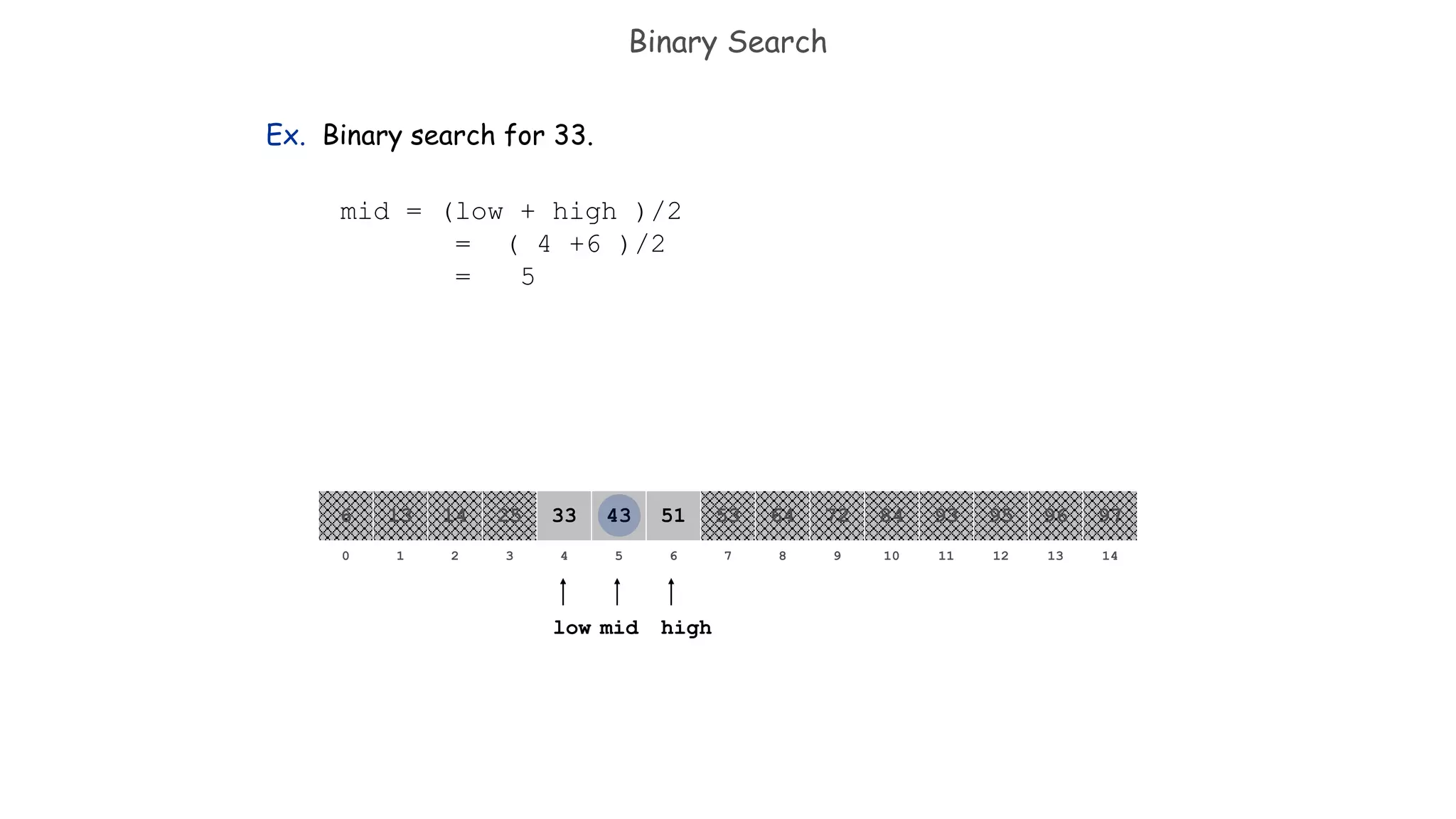
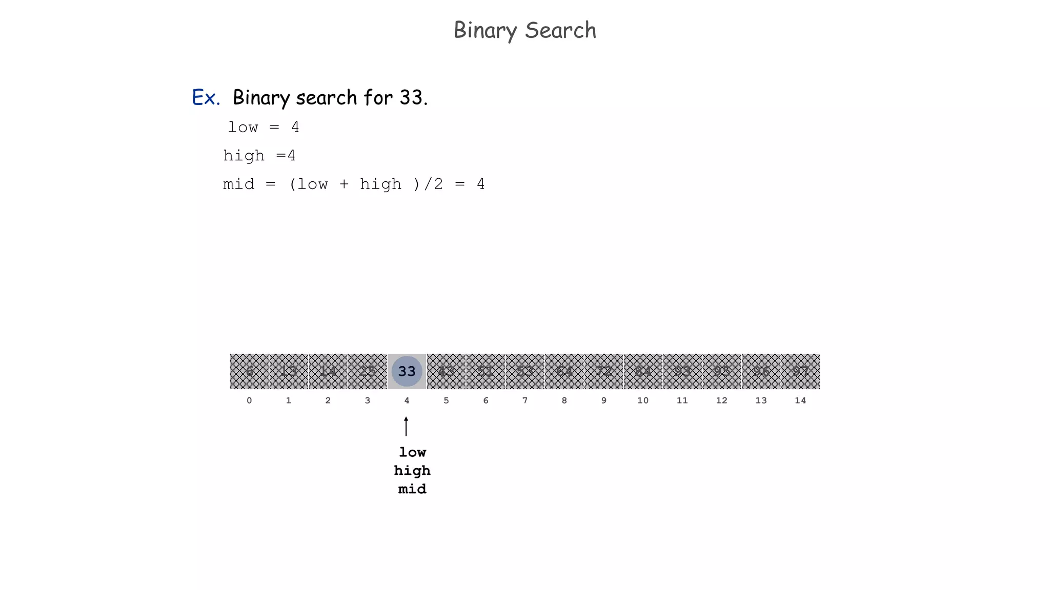
![Binary Search
Ex. Binary search for 33.
821 3 4 65 7 109 11 12 14130
641413 25 33 5143 53 8472 93 95 97966
low high
Since key < A [mid],
Update: high = mid -1
Low = 0
High = 6](https://image.slidesharecdn.com/unit-8searchingandhashing-171201035421/75/Unit-8-searching-and-hashing-11-2048.jpg)
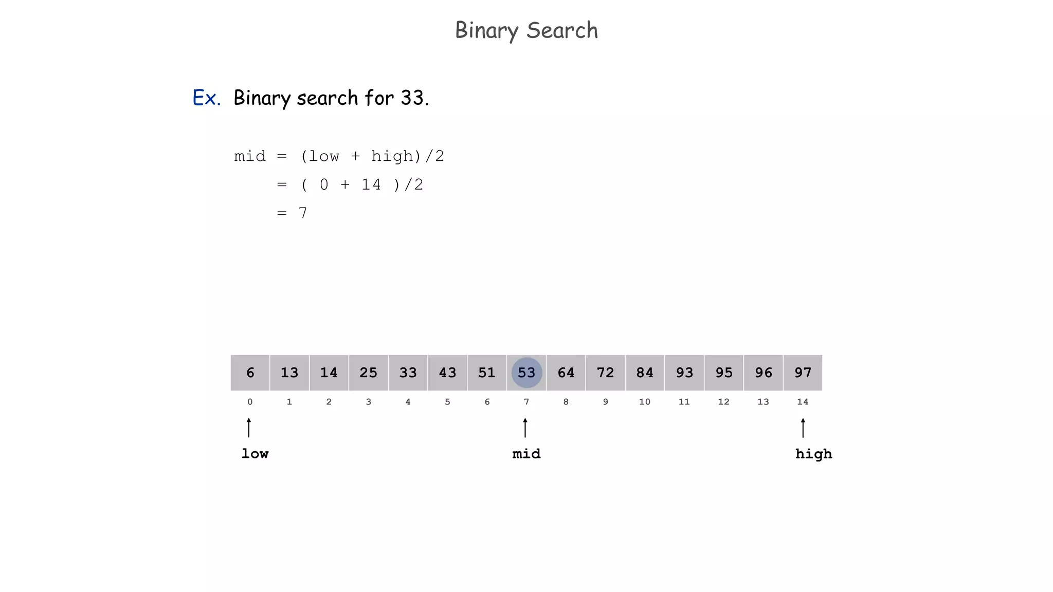
![Binary Search
Ex. Binary search for 33.
821 3 4 65 7 109 11 12 14130
641413 25 33 5143 53 8472 93 95 97966
low high
Since key > A [mid],
Update: low = mid +1](https://image.slidesharecdn.com/unit-8searchingandhashing-171201035421/75/Unit-8-searching-and-hashing-13-2048.jpg)
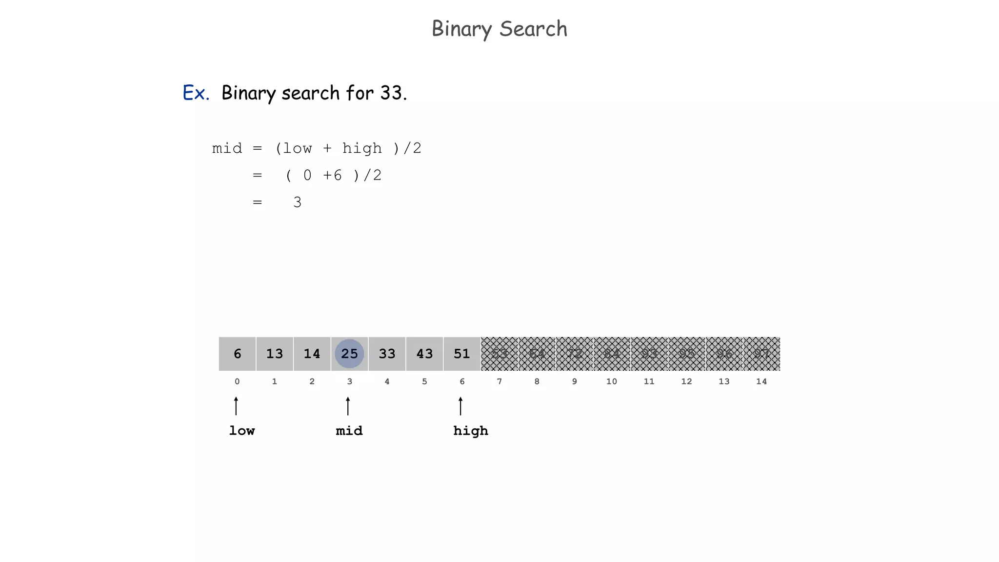
![Binary Search
Ex. Binary search for 33.
821 3 4 65 7 109 11 12 14130
641413 25 33 5143 53 8472 93 95 97966
low
high
Since key < A [mid],
Update: low = mid -1](https://image.slidesharecdn.com/unit-8searchingandhashing-171201035421/75/Unit-8-searching-and-hashing-15-2048.jpg)
![Binary Search
Ex. Binary search for 33.
a[mid] = 33
search successful !!
821 3 4 65 7 109 11 12 14130
641413 25 33 5143 53 8472 93 95 97966
low
high
mid](https://image.slidesharecdn.com/unit-8searchingandhashing-171201035421/75/Unit-8-searching-and-hashing-17-2048.jpg)
![18
Trace Binary Search
Take input array a[]
For Search key = 2
l r mid remarks
0 13 6 Key < a[6] i.e. 2 < 53
0 5 2 Key < a[2] i.e. 2 < 7
0 1 0 Key == a[0] i.e. 2 ==a[0]
Therefore, key found at index 0.
Search Successful !!
2 5 7 9 18 45 53 59 67 72 88 95 101 104
0 1 2 3 4 5 6 7 8 9 10 11 12 13
Exercise : Trace binary search algorithm for keys:
i. 67
ii. 50
iii. 250](https://image.slidesharecdn.com/unit-8searchingandhashing-171201035421/75/Unit-8-searching-and-hashing-18-2048.jpg)
![19
Search for key = 67
l r mid Remarks
0 13 6 Key < a[6] i.e. 67 > 53
7 13 10 Key < a[10] i.e. 67 < 88
7 9 8 Key == a[8] i.e. 67 ==a[8]
Therefore, key found at index 8.
Search Successful !!
2 5 7 9 18 45 53 59 67 72 88 95 101 104
0 1 2 3 4 5 6 7 8 9 10 11 12 13
Input Array : a[ ]](https://image.slidesharecdn.com/unit-8searchingandhashing-171201035421/75/Unit-8-searching-and-hashing-19-2048.jpg)
![20
Search for key = 50
l r mid Remarks
0 13 6 Key < a[6] i.e. 50 < 53
0 5 2 Key < a[2] i.e. 50 > 7
3 5 4 Key > a[4] i.e. 50 >18
5 5 5 Key > a[5] i.e. 50 > 45
6 5 l > r, terminate
Therefore, key not found in the array.
Search Unsuccessful !!
2 5 7 9 18 45 53 59 67 72 88 95 101 104
0 1 2 3 4 5 6 7 8 9 10 11 12 13
Given Input Array a[]](https://image.slidesharecdn.com/unit-8searchingandhashing-171201035421/75/Unit-8-searching-and-hashing-20-2048.jpg)
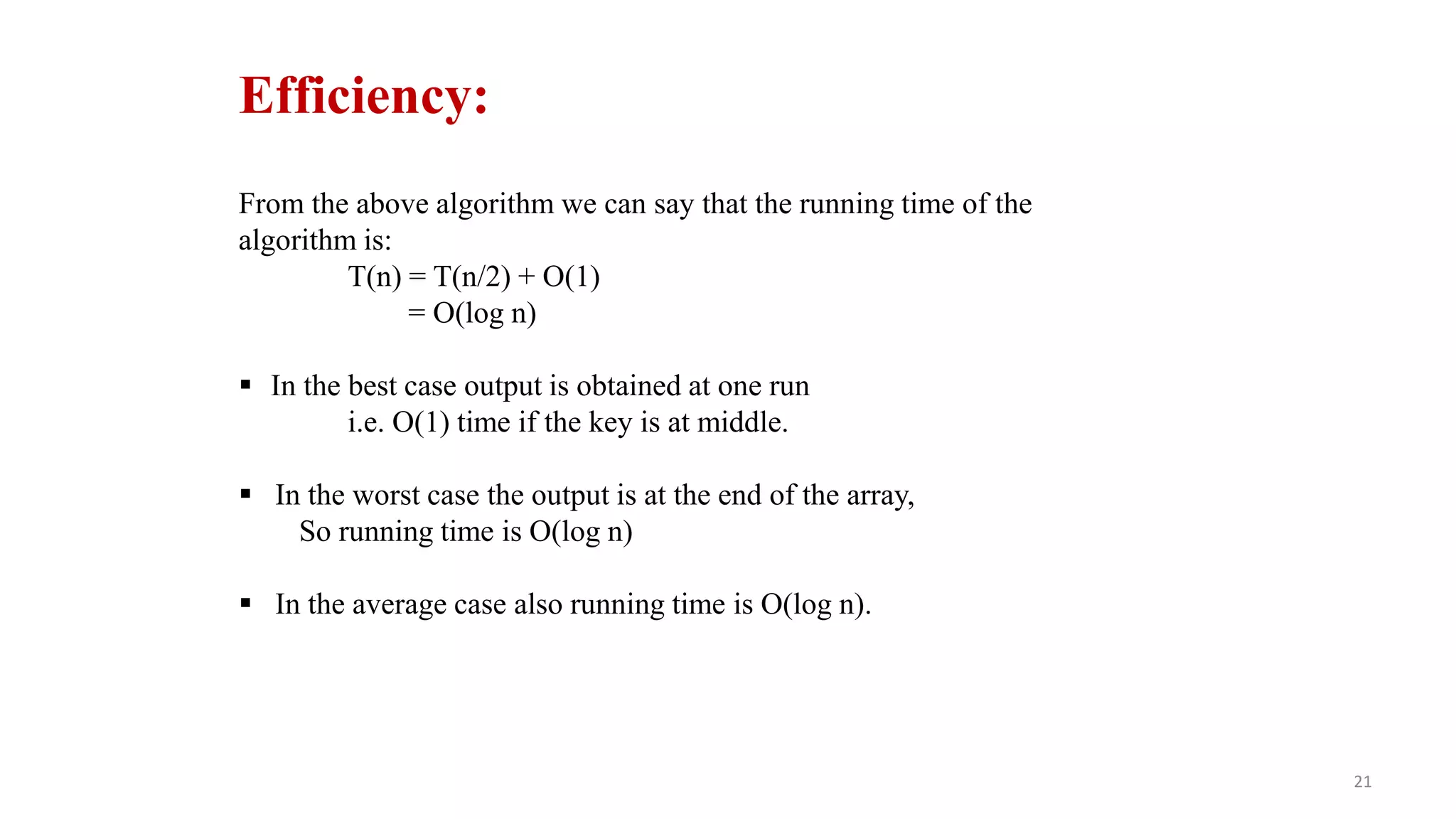
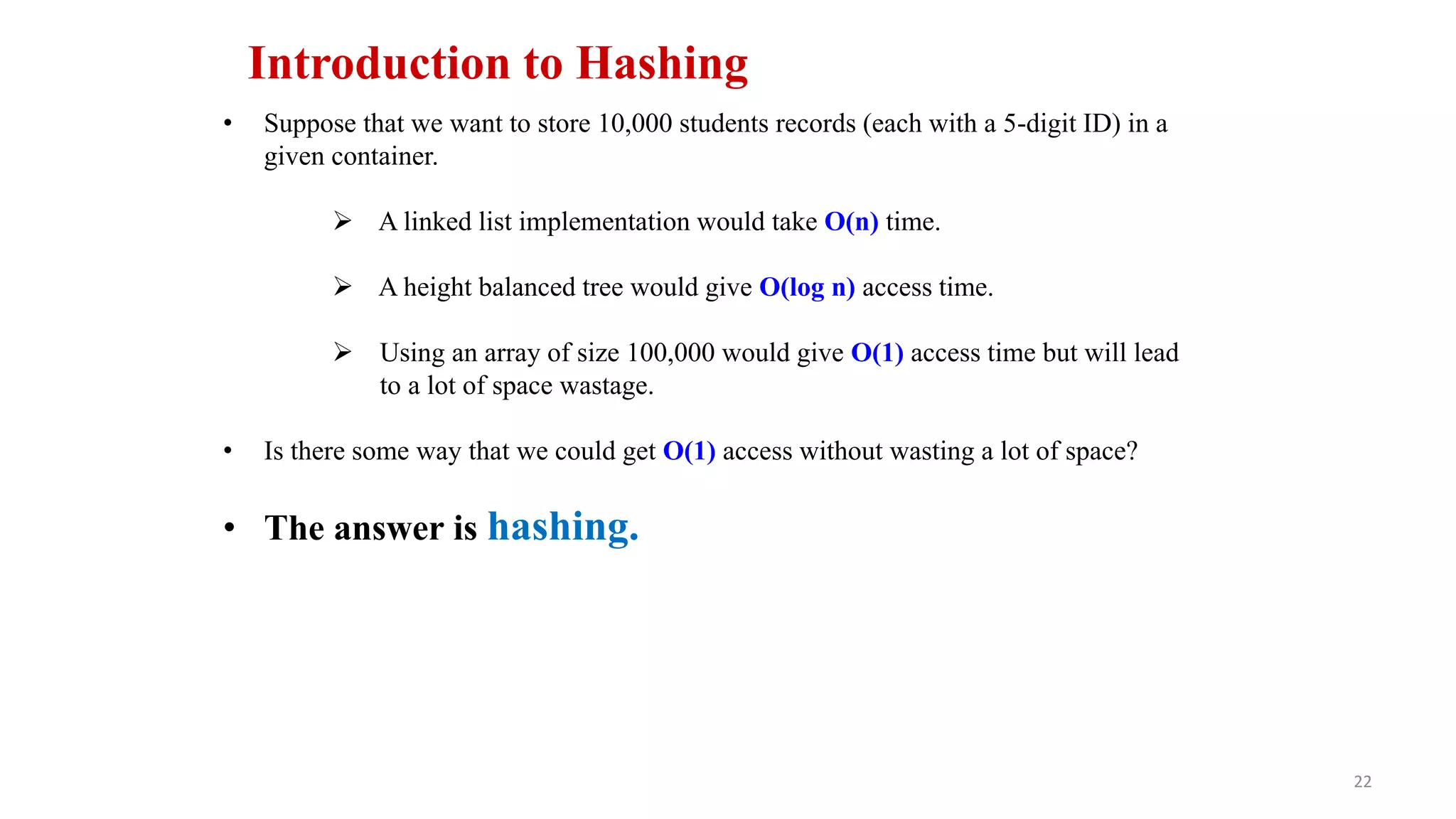
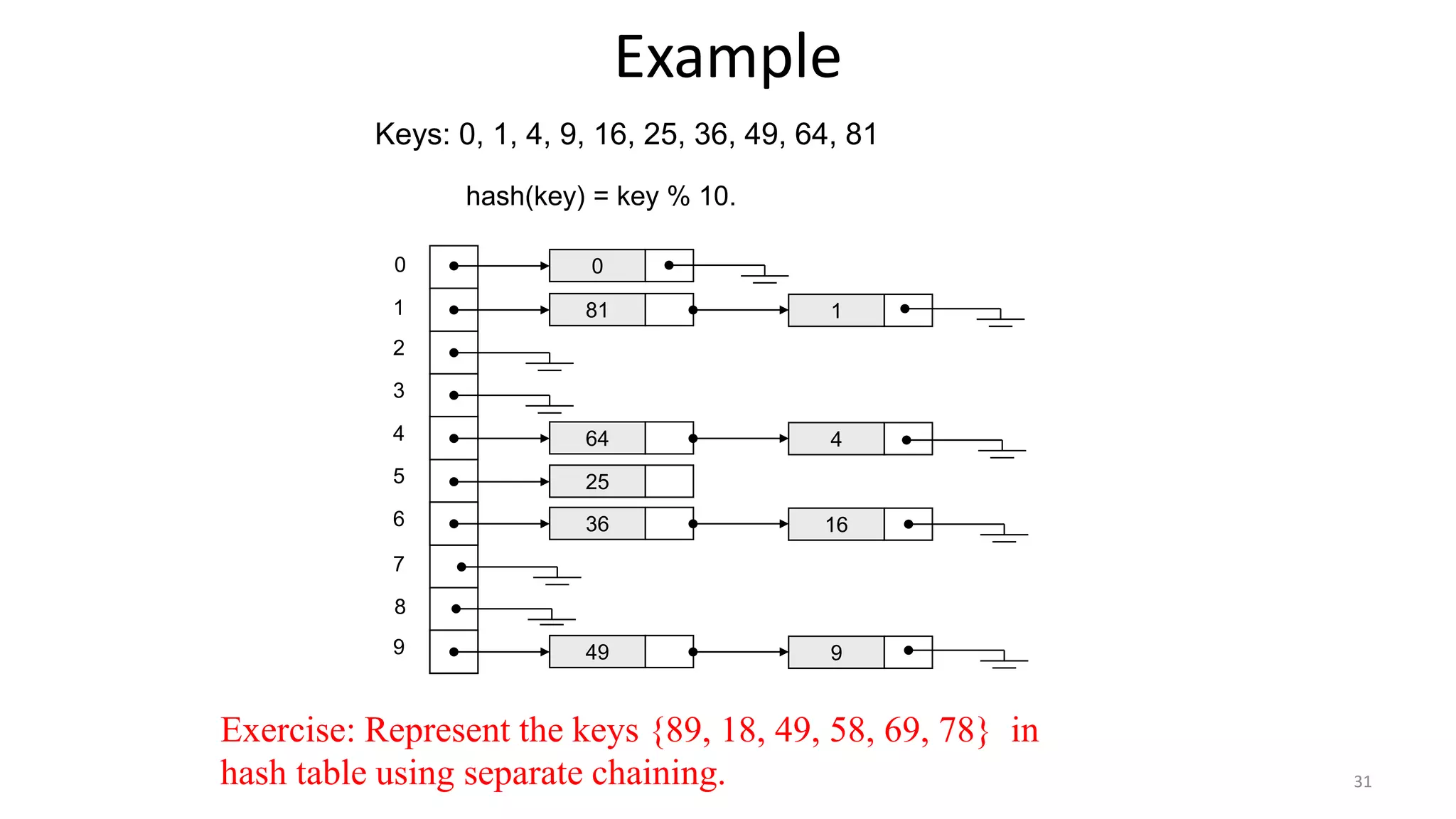


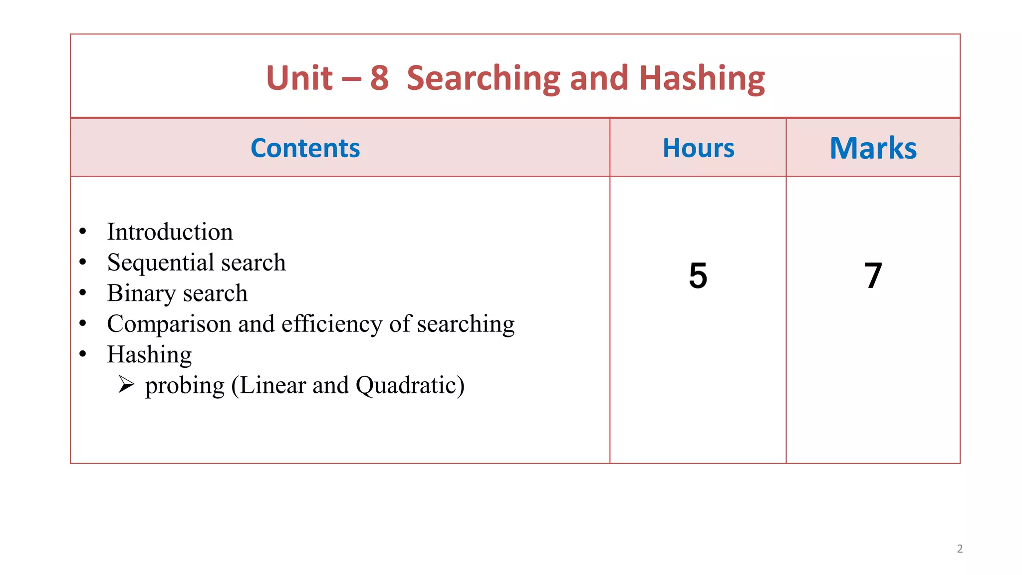
1. The document discusses searching and hashing algorithms. It describes linear and binary searching techniques. Linear search has O(n) time complexity, while binary search has O(log n) time complexity for sorted arrays. 2. Hashing is described as a technique to allow O(1) access time by mapping keys to table indexes via a hash function. Separate chaining and open addressing are two common techniques for resolving collisions when different keys hash to the same index. Separate chaining uses linked lists at each table entry while open addressing probes for the next open slot.
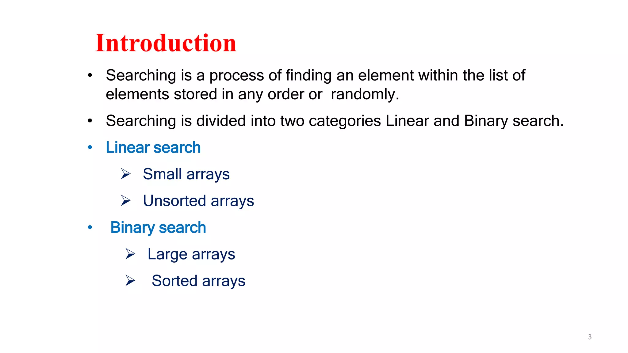
Introduction to Searching and Hashing, covering Linear and Binary search techniques.
Explains linear search, its algorithm, and time complexity, suitable for small and unsorted arrays.
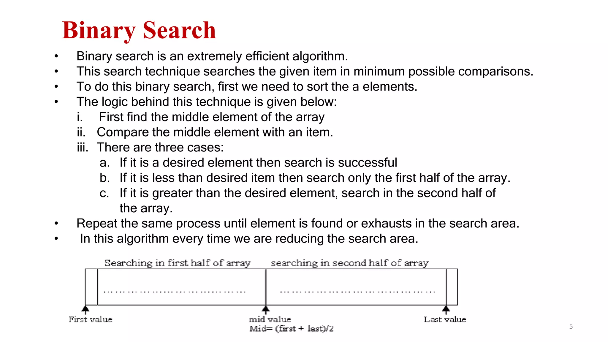
Details of binary search techniques with algorithms (iterative and recursive), efficient for sorted arrays.
Demonstrates a binary search example for the key 33 with step-by-step access and results.
Describes tracing binary search for keys 2, 67, and 50, assessing their outcomes.
Analyzes binary search's efficiency with time complexity being O(log n) across various scenarios.
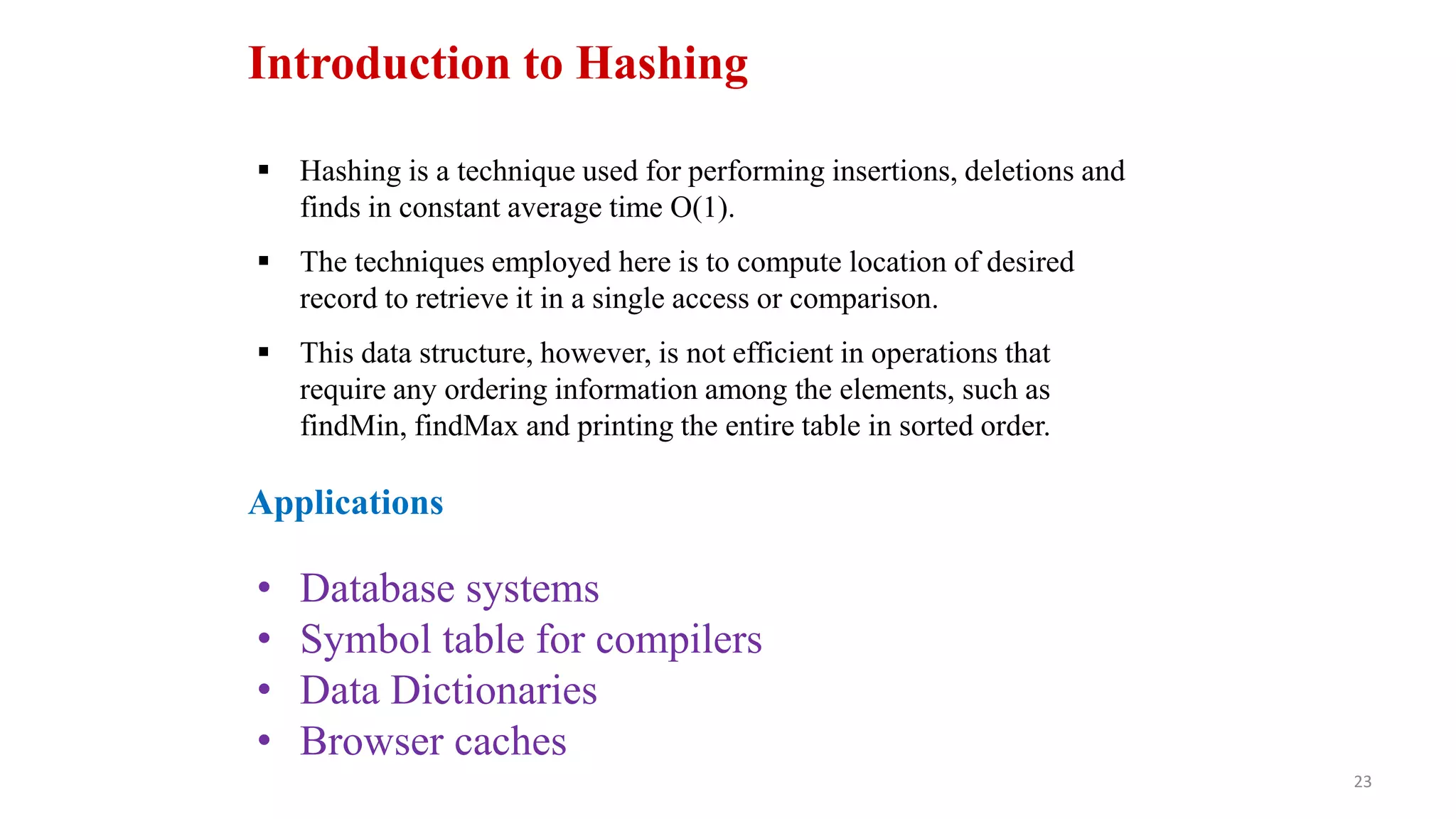
Introduction to hashing, its advantages for record access, and its common applications.
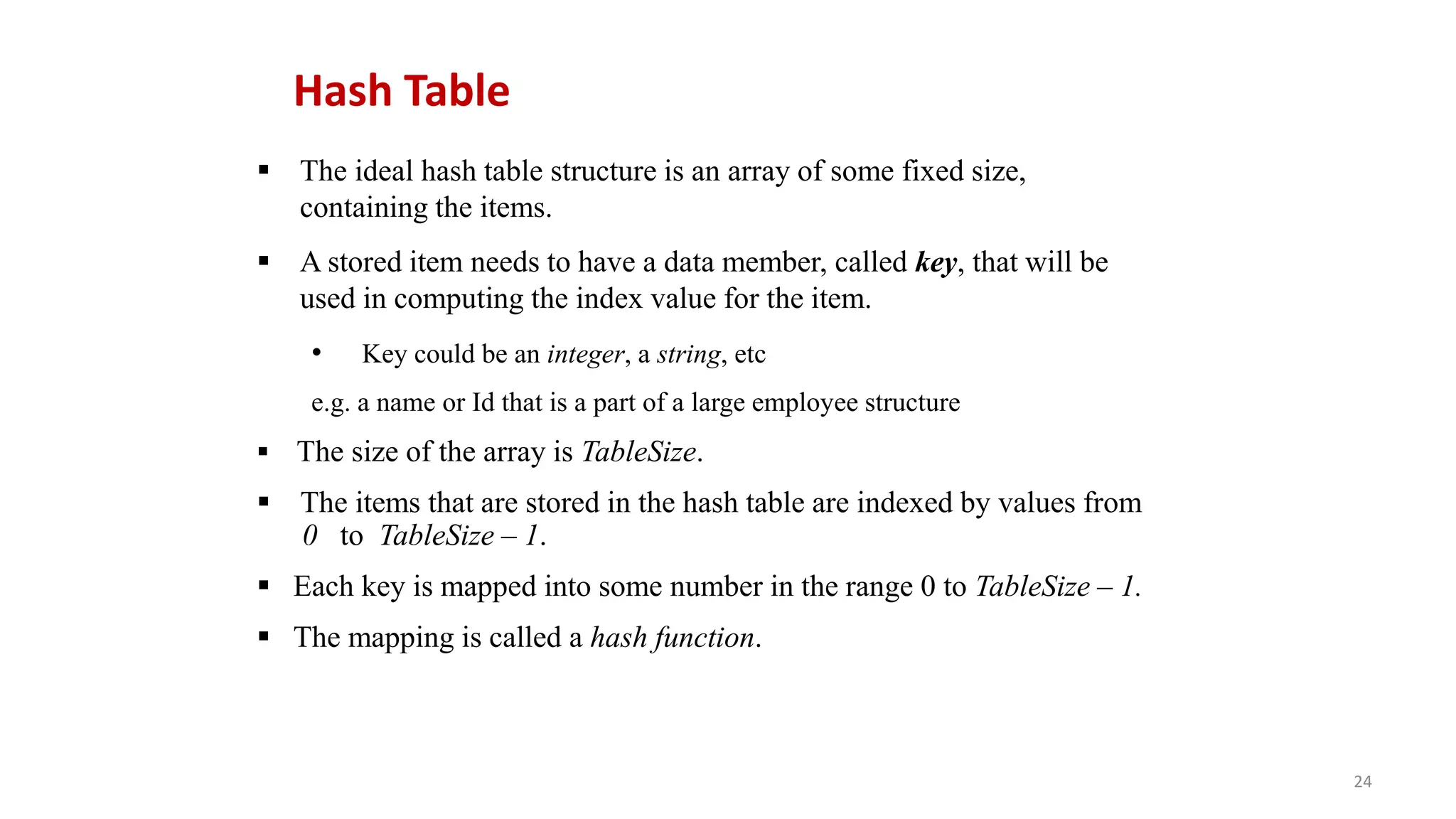
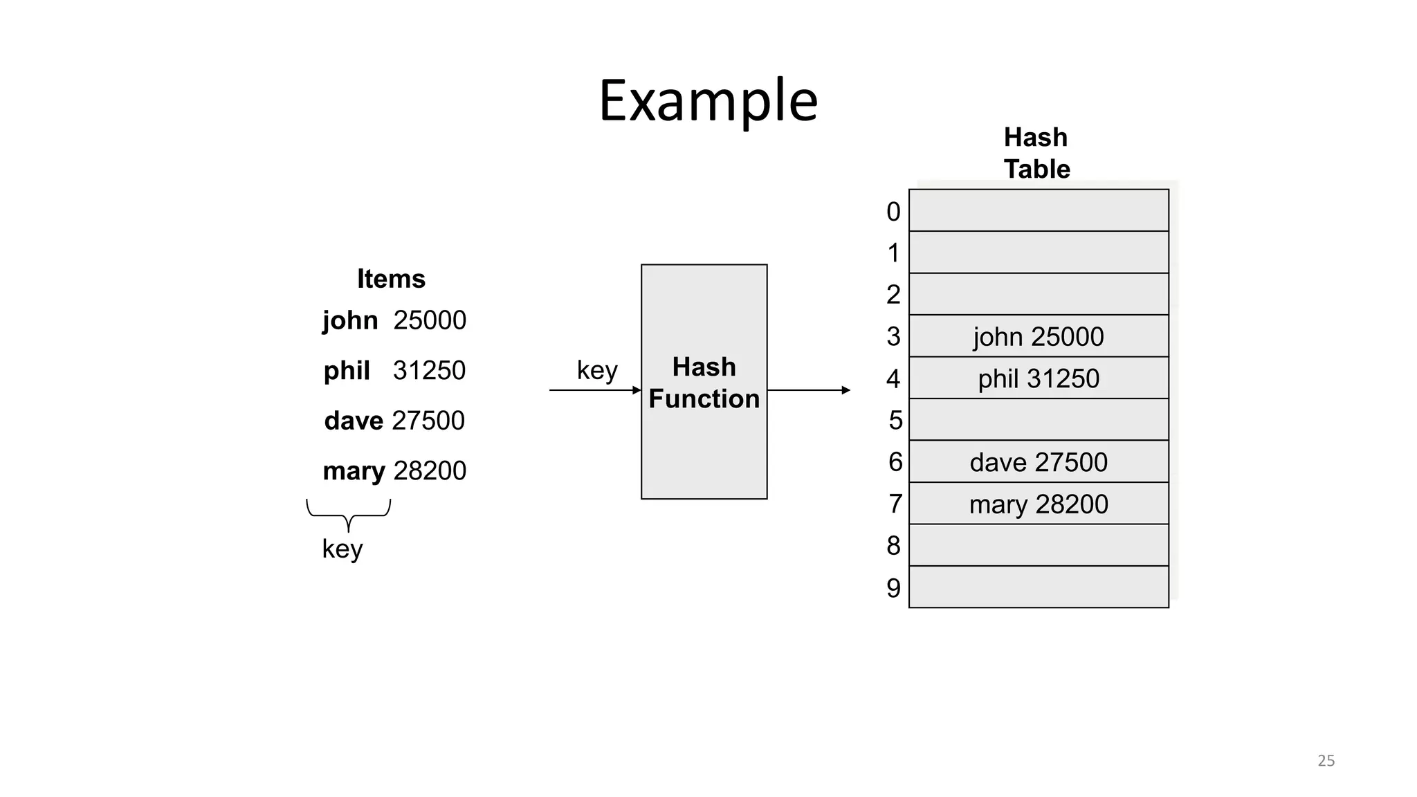
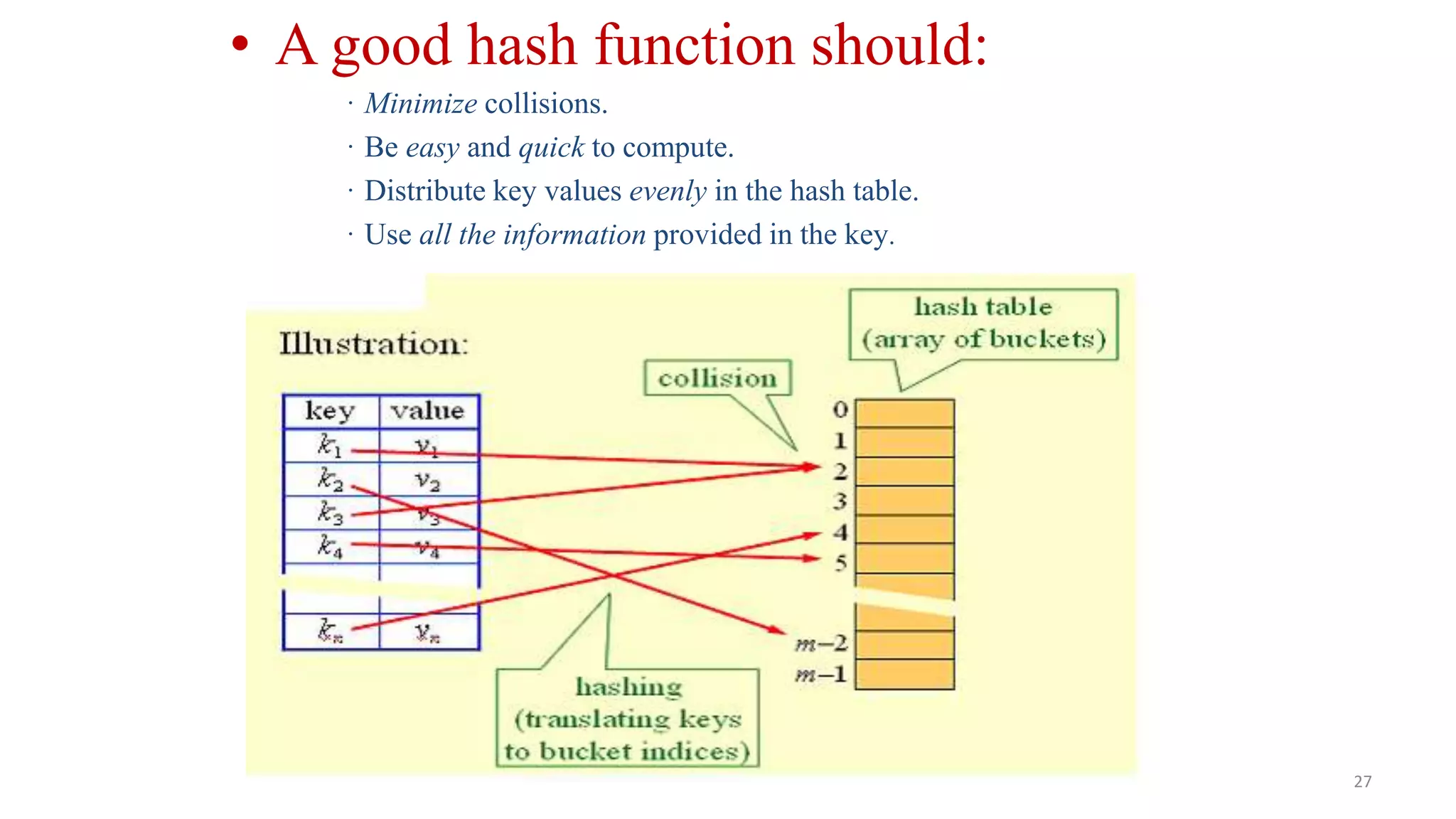
Describes ideal hash table structure, mapping keys to indices using hash functions, showcasing examples.
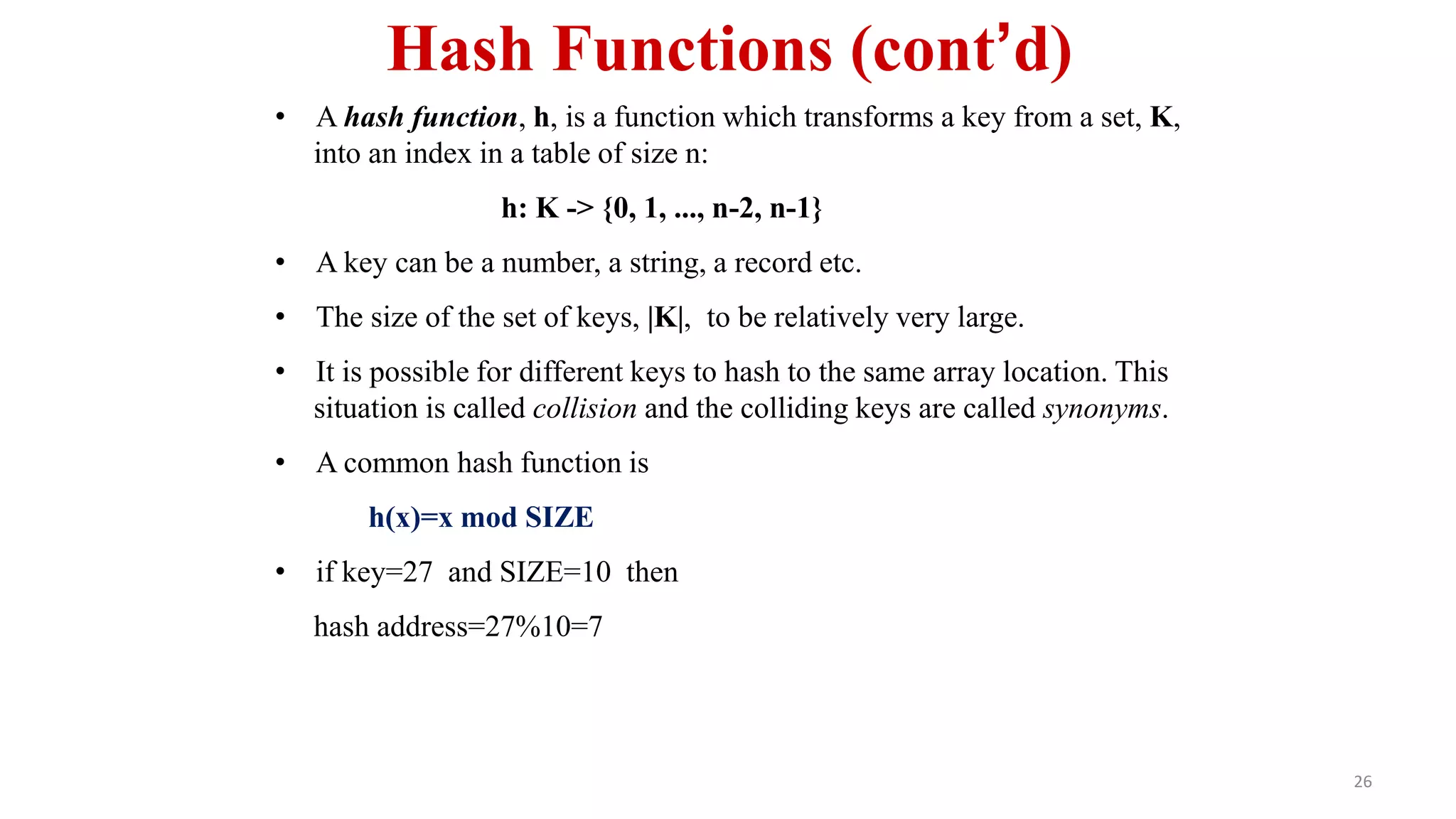
Details on hash functions, addressing collisions through synonyms, and characteristics of good functions.
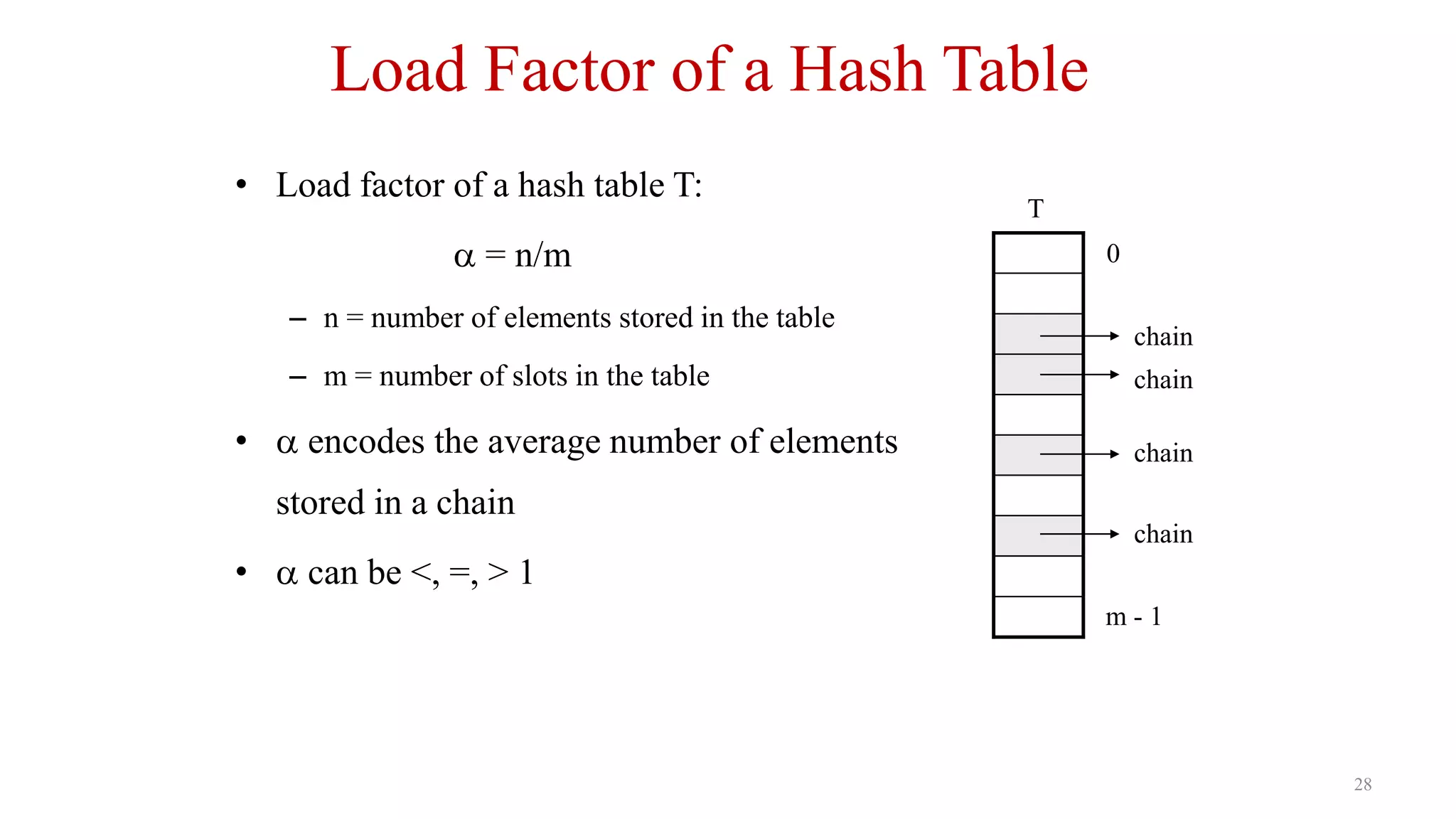
Defines load factor in hash tables, implications of n/m ratio for efficient storage performance.
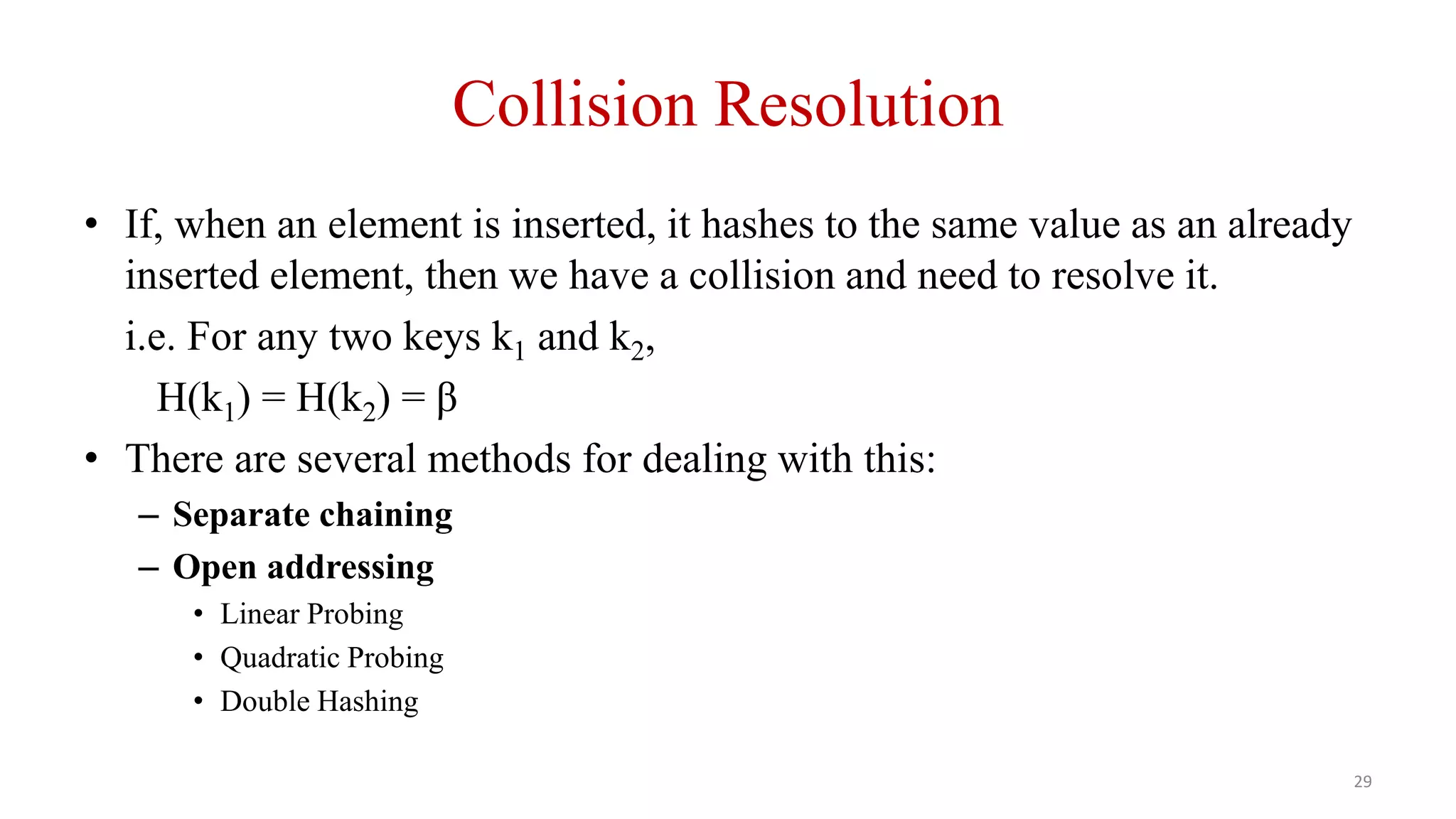
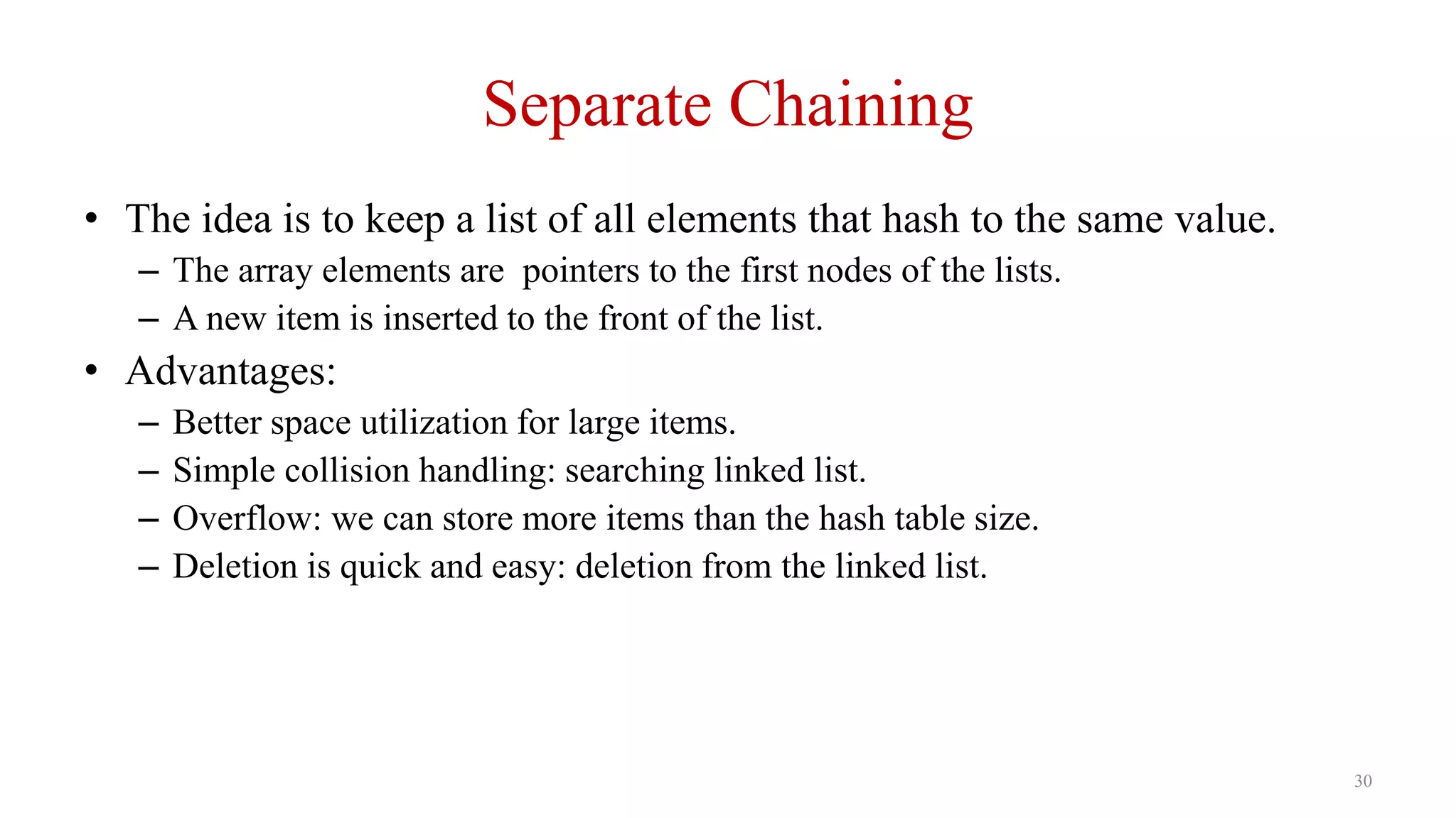
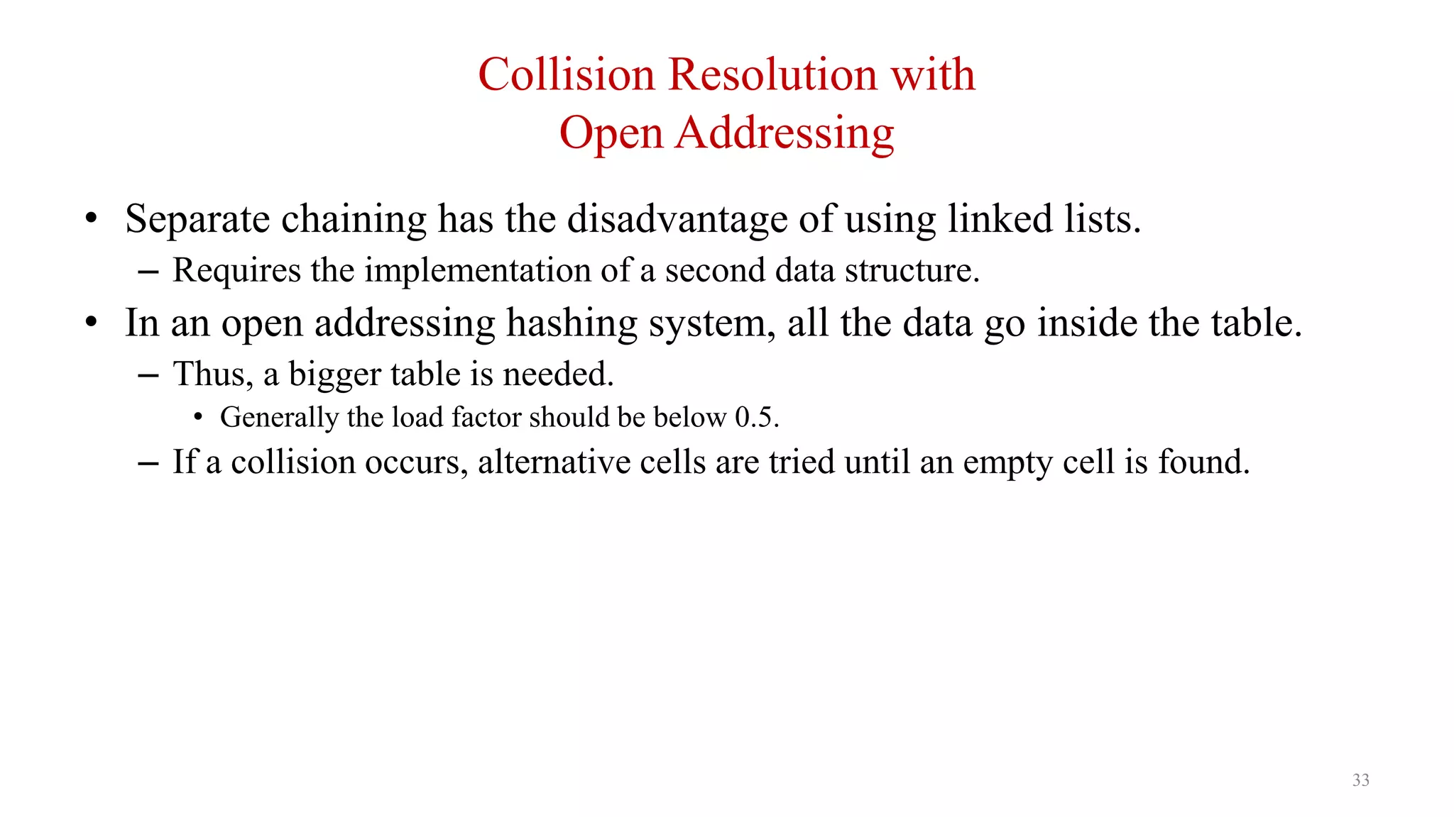
Explains collision resolution techniques like separate chaining with pros and operational methods.
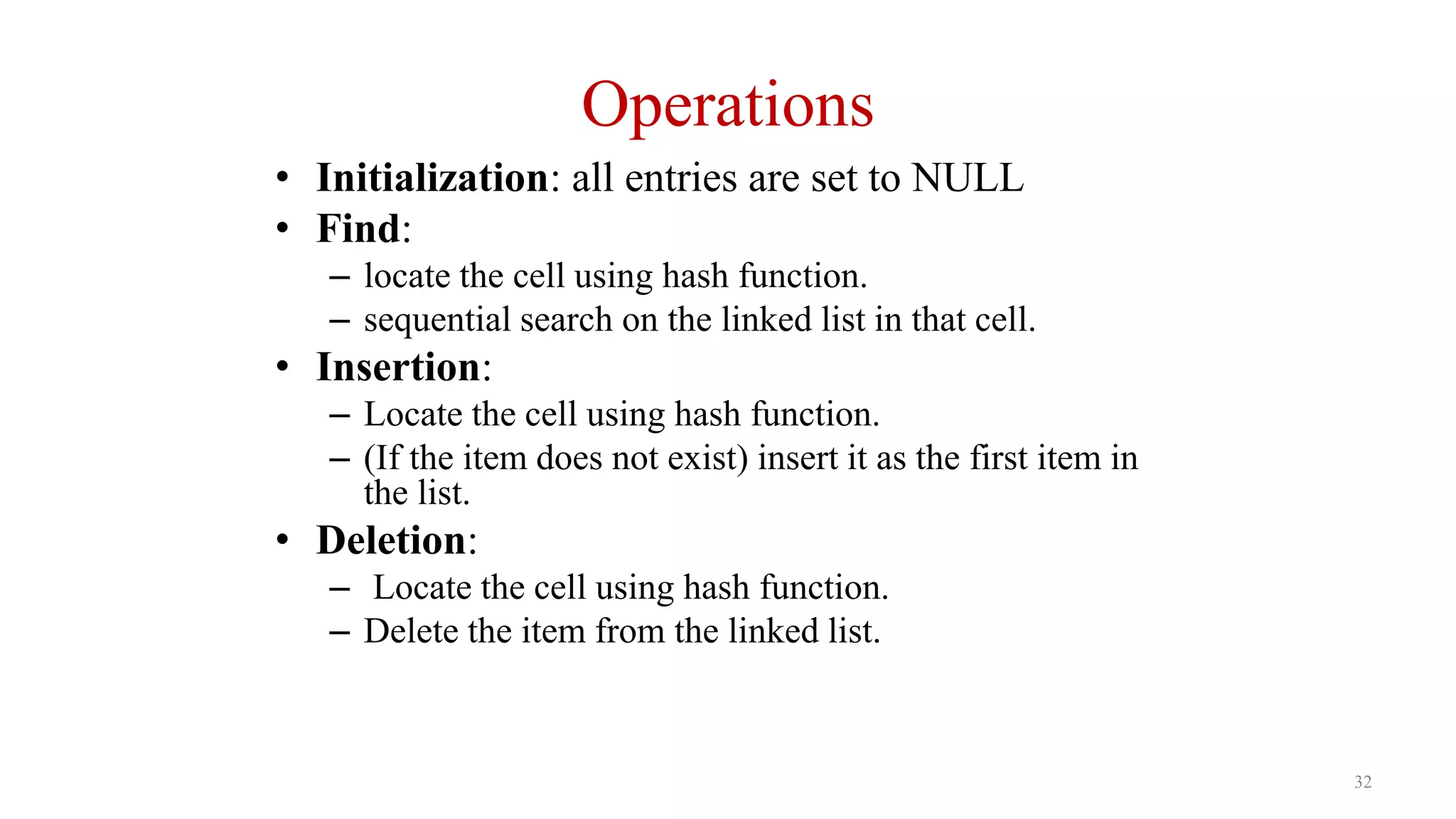
Outlines initialization, searching, insertion, and deletion processes in hash tables.
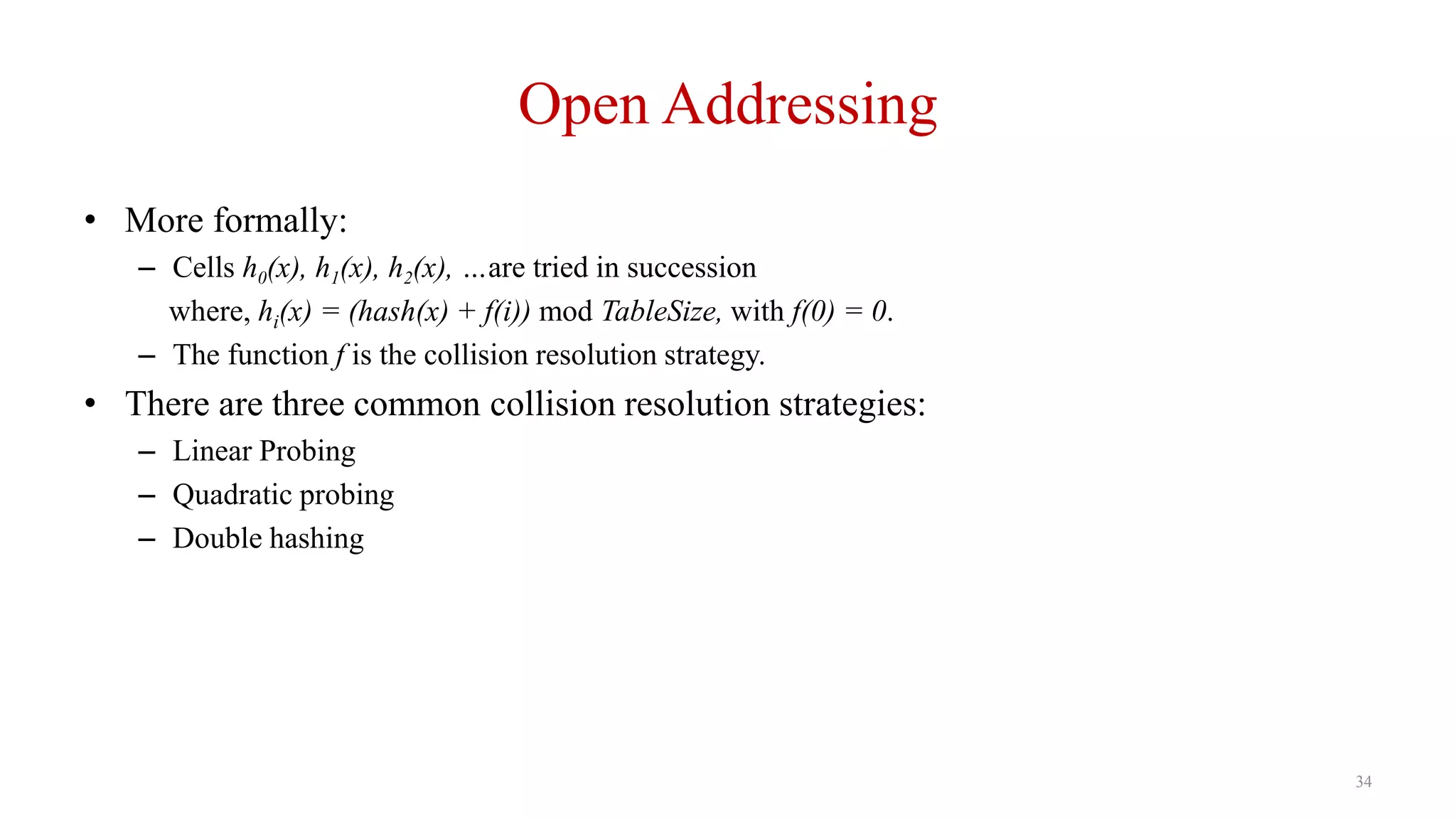
Explains open addressing for collision resolution and strategies like linear and quadratic probing.
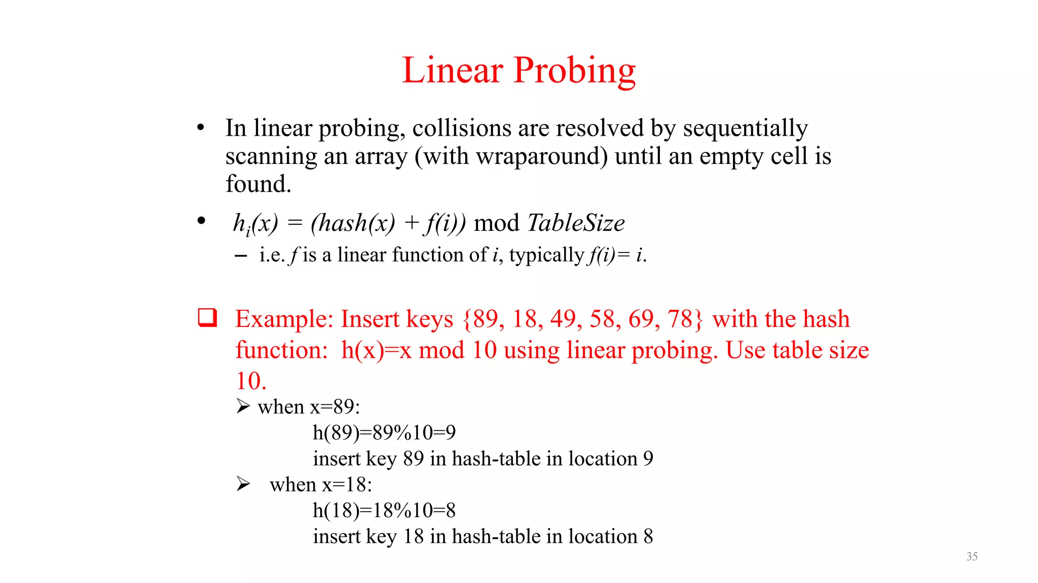
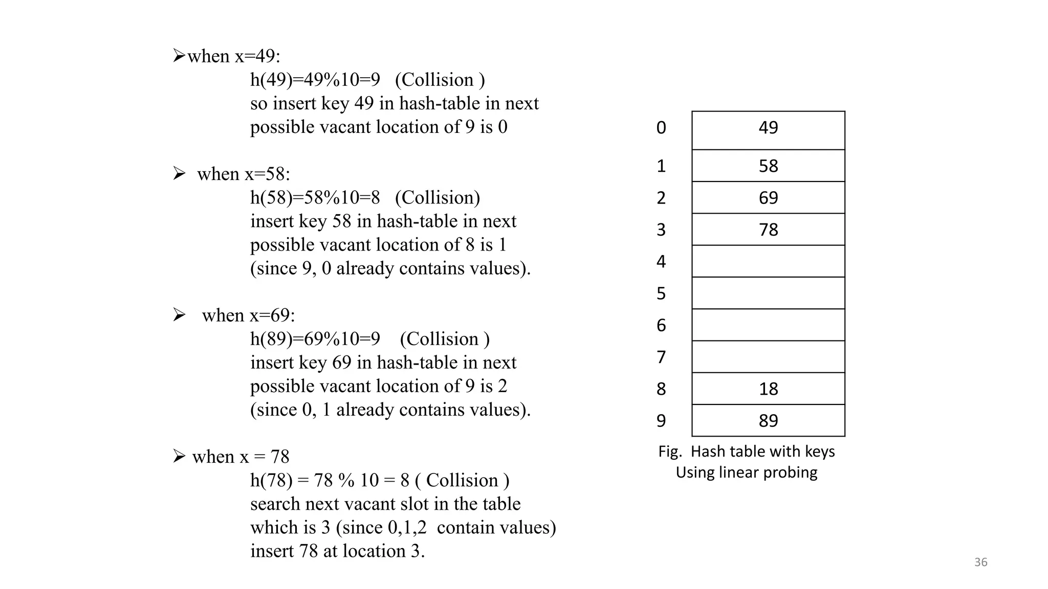
Details on the linear probing technique for collision resolution and its implementation examples.
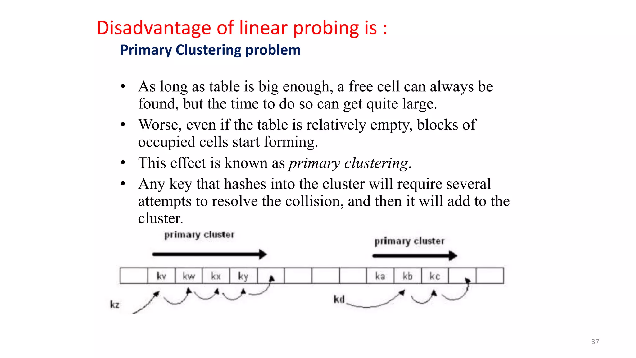
Explains primary clustering issue in linear probing, leading to increased search time.
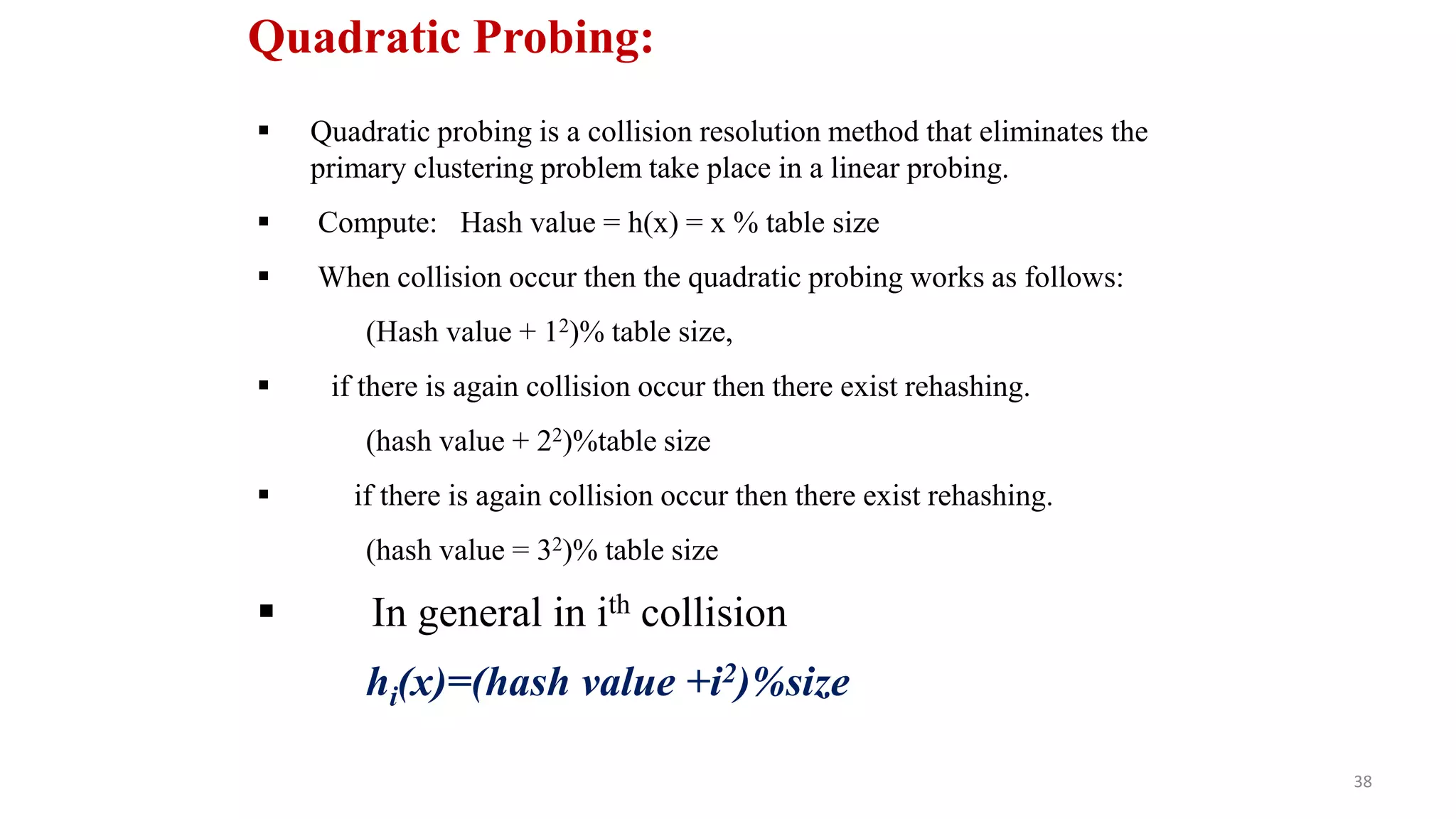
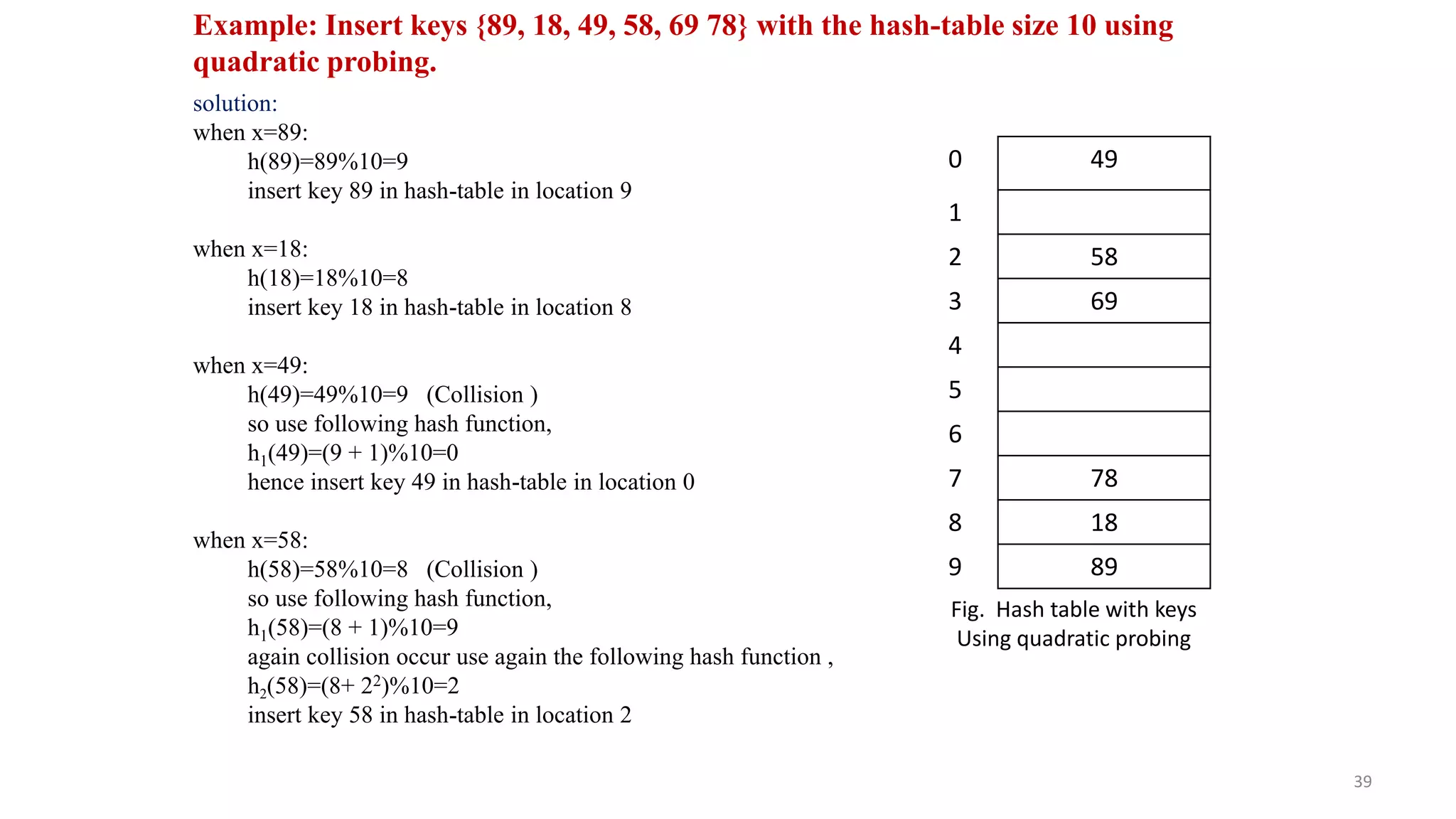
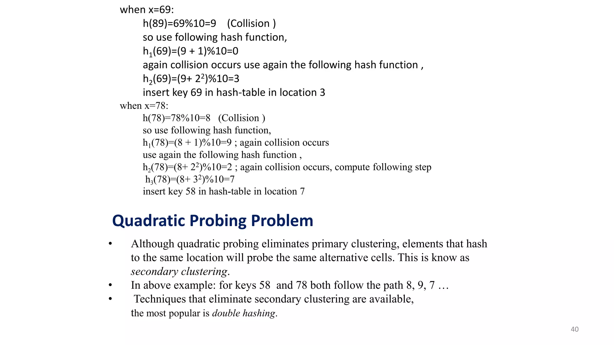
Explains quadratic probing as a collision resolution method and addresses secondary clustering.
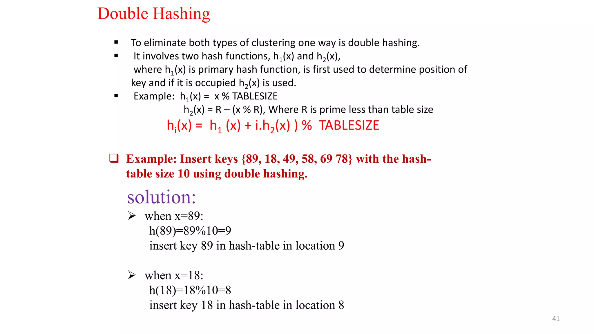
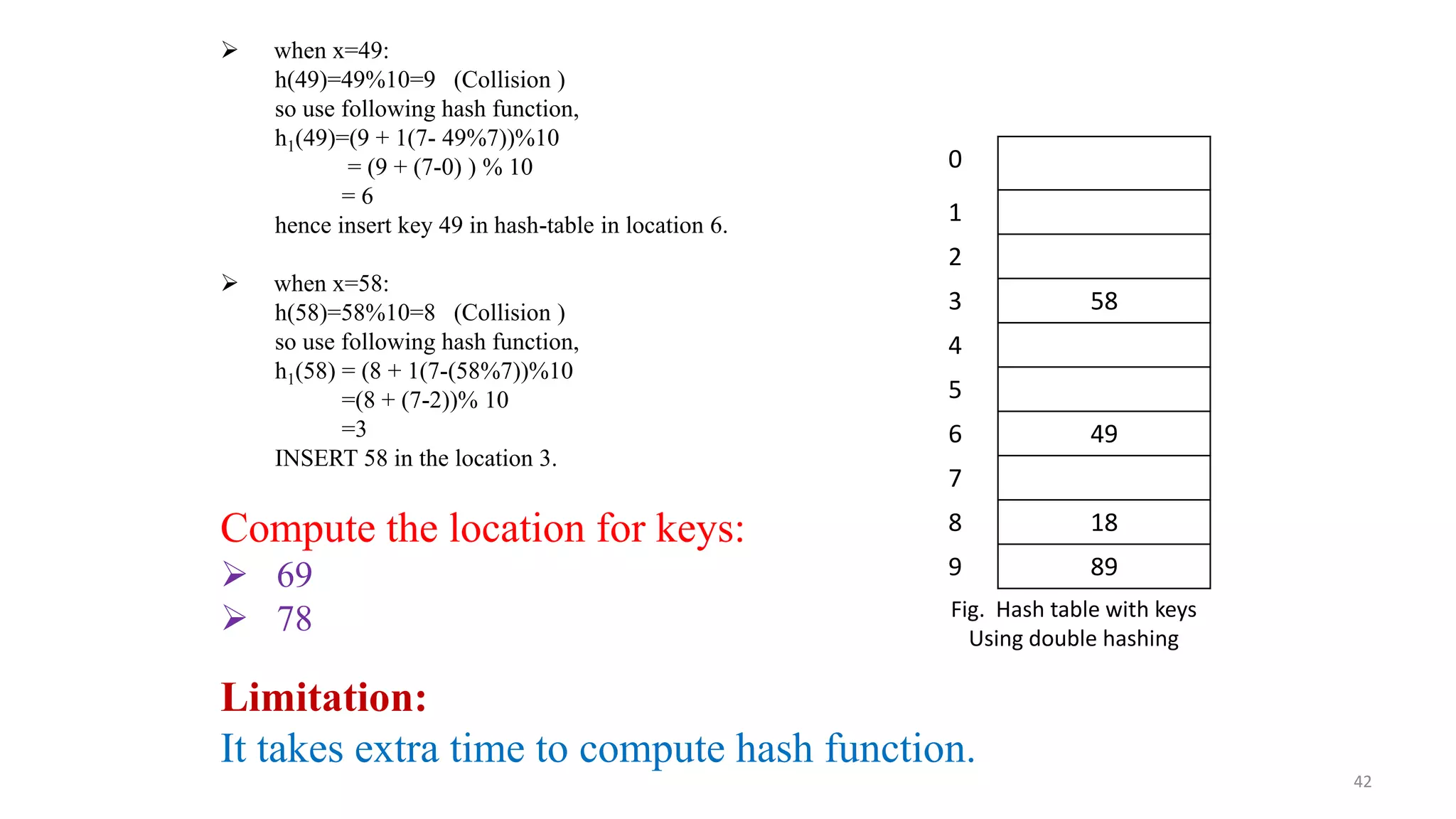
Introduces double hashing to resolve clustering issues with two hash functions and provides examples.


![ANPARA THERMAL POWER STATION[1] sangam.pdf](https://cdn.slidesharecdn.com/ss_thumbnails/anparathermalpowerstation1sangam-251121115219-9261cde4-thumbnail.jpg?width=640&height=640&fit=bounds)


