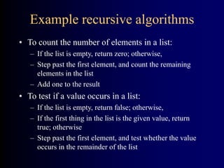
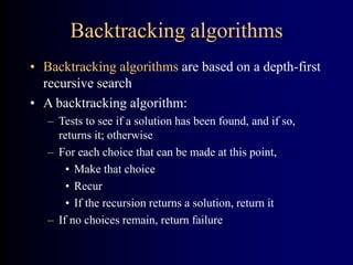
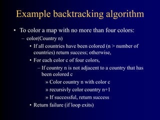
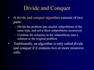
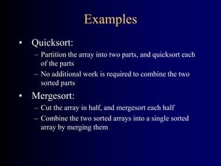
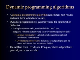
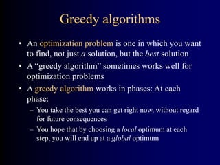
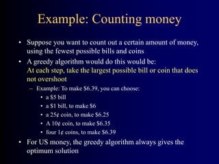
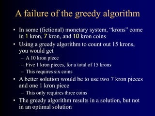
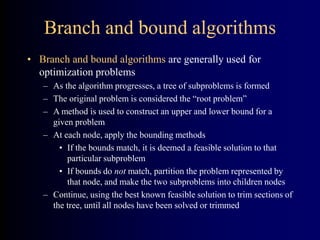
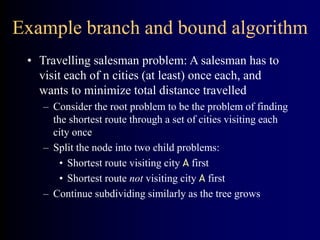
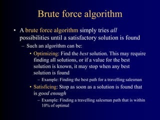
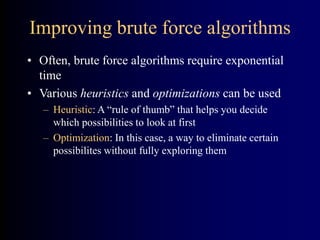
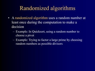
This document discusses different types of algorithms. It provides examples of:
- Simple recursive algorithms that solve base cases and recursively call simpler subproblems.
- Backtracking algorithms that use depth-first search and backtrack when choices lead to dead ends.
- Divide and conquer algorithms that divide problems into subproblems, solve the subproblems recursively, and combine the solutions.
- Dynamic programming algorithms that store and reuse solutions to overlapping subproblems to optimize problems.
- Greedy algorithms that make locally optimal choices at each step to hopefully find a global optimum.
- Branch and bound algorithms that construct a search tree and prune suboptimal branches.
- Brute force algorithms that exhaustively check all possibilities until finding a solution
Design and Analysis of Algorithm help to design the algorithms for solving different types of problems in Computer Science. It also helps to design and analyze the logic of how the program will work before developing the actual code for a program.
2. Algorithm classification
• Algorithms that use a similar problem-solving
approach can be grouped together
• This classification scheme is neither exhaustive
nor disjoint
• The purpose is not to be able to classify an
algorithm as one type or another, but to highlight
the various ways in which a problem can be
attacked
3. A short list of categories
• Algorithm types we will consider include:
– Simple recursive algorithms
– Backtracking algorithms
– Divide and conquer algorithms
– Dynamic programming algorithms
– Greedy algorithms
– Branch and bound algorithms
– Brute force algorithms
– Randomized algorithms
4. Simple recursive algorithms I
• A simple recursive algorithm:
– Solves the base cases directly
– Recurs with a simpler subproblem
– Does some extra work to convert the solution to the
simpler subproblem into a solution to the given
problem
• I call these “simple” because several of the other
algorithm types are inherently recursive
5. Example recursive algorithms
• To count the number of elements in a list:
– If the list is empty, return zero; otherwise,
– Step past the first element, and count the remaining
elements in the list
– Add one to the result
• To test if a value occurs in a list:
– If the list is empty, return false; otherwise,
– If the first thing in the list is the given value, return
true; otherwise
– Step past the first element, and test whether the value
occurs in the remainder of the list
6. Backtracking algorithms
• Backtracking algorithms are based on a depth-first
recursive search
• A backtracking algorithm:
– Tests to see if a solution has been found, and if so,
returns it; otherwise
– For each choice that can be made at this point,
• Make that choice
• Recur
• If the recursion returns a solution, return it
– If no choices remain, return failure
7. Example backtracking algorithm
• To color a map with no more than four colors:
– color(Country n)
• If all countries have been colored (n > number of
countries) return success; otherwise,
• For each color c of four colors,
– If country n is not adjacent to a country that has
been colored c
» Color country n with color c
» recursivly color country n+1
» If successful, return success
• Return failure (if loop exits)
8. Divide and Conquer
• A divide and conquer algorithm consists of two
parts:
– Divide the problem into smaller subproblems of the
same type, and solve these subproblems recursively
– Combine the solutions to the subproblems into a
solution to the original problem
• Traditionally, an algorithm is only called divide
and conquer if it contains two or more recursive
calls
9. Examples
• Quicksort:
– Partition the array into two parts, and quicksort each
of the parts
– No additional work is required to combine the two
sorted parts
• Mergesort:
– Cut the array in half, and mergesort each half
– Combine the two sorted arrays into a single sorted
array by merging them
10. Binary tree lookup
• Here’s how to look up something in a sorted
binary tree:
– Compare the key to the value in the root
• If the two values are equal, report success
• If the key is less, search the left subtree
• If the key is greater, search the right subtree
• This is not a divide and conquer algorithm
because, although there are two recursive calls,
only one is used at each level of the recursion
11. Fibonacci numbers
• To find the nth Fibonacci number:
– If n is zero or one, return one; otherwise,
– Compute fibonacci(n-1) and fibonacci(n-2)
– Return the sum of these two numbers
• This is an expensive algorithm
– It requires O(fibonacci(n)) time
– This is equivalent to exponential time, that is, O(2n)
12. Dynamic programming algorithms
• A dynamic programming algorithm remembers past results
and uses them to find new results
• Dynamic programming is generally used for optimization
problems
– Multiple solutions exist, need to find the “best” one
– Requires “optimal substructure” and “overlapping subproblems”
• Optimal substructure: Optimal solution contains optimal
solutions to subproblems
• Overlapping subproblems: Solutions to subproblems can be
stored and reused in a bottom-up fashion
• This differs from Divide and Conquer, where subproblems
generally need not overlap
13. Fibonacci numbers again
• To find the nth Fibonacci number:
– If n is zero or one, return one; otherwise,
– Compute, or look up in a table, fibonacci(n-1) and
fibonacci(n-2)
– Find the sum of these two numbers
– Store the result in a table and return it
• Since finding the nth Fibonacci number involves
finding all smaller Fibonacci numbers, the second
recursive call has little work to do
• The table may be preserved and used again later
14. Greedy algorithms
• An optimization problem is one in which you want
to find, not just a solution, but the best solution
• A “greedy algorithm” sometimes works well for
optimization problems
• A greedy algorithm works in phases: At each
phase:
– You take the best you can get right now, without regard
for future consequences
– You hope that by choosing a local optimum at each
step, you will end up at a global optimum
15. Example: Counting money
• Suppose you want to count out a certain amount of money,
using the fewest possible bills and coins
• A greedy algorithm would do this would be:
At each step, take the largest possible bill or coin that does
not overshoot
– Example: To make $6.39, you can choose:
• a $5 bill
• a $1 bill, to make $6
• a 25¢ coin, to make $6.25
• A 10¢ coin, to make $6.35
• four 1¢ coins, to make $6.39
• For US money, the greedy algorithm always gives the
optimum solution
16. A failure of the greedy algorithm
• In some (fictional) monetary system, “krons” come
in 1 kron, 7 kron, and 10 kron coins
• Using a greedy algorithm to count out 15 krons,
you would get
– A 10 kron piece
– Five 1 kron pieces, for a total of 15 krons
– This requires six coins
• A better solution would be to use two 7 kron pieces
and one 1 kron piece
– This only requires three coins
• The greedy algorithm results in a solution, but not
in an optimal solution
17. Branch and bound algorithms
• Branch and bound algorithms are generally used for
optimization problems
– As the algorithm progresses, a tree of subproblems is formed
– The original problem is considered the “root problem”
– A method is used to construct an upper and lower bound for a
given problem
– At each node, apply the bounding methods
• If the bounds match, it is deemed a feasible solution to that
particular subproblem
• If bounds do not match, partition the problem represented by
that node, and make the two subproblems into children nodes
– Continue, using the best known feasible solution to trim sections of
the tree, until all nodes have been solved or trimmed
18. Example branch and bound algorithm
• Travelling salesman problem: A salesman has to
visit each of n cities (at least) once each, and
wants to minimize total distance travelled
– Consider the root problem to be the problem of finding
the shortest route through a set of cities visiting each
city once
– Split the node into two child problems:
• Shortest route visiting city A first
• Shortest route not visiting city A first
– Continue subdividing similarly as the tree grows
19. Brute force algorithm
• A brute force algorithm simply tries all
possibilities until a satisfactory solution is found
– Such an algorithm can be:
• Optimizing: Find the best solution. This may require
finding all solutions, or if a value for the best
solution is known, it may stop when any best
solution is found
– Example: Finding the best path for a travelling salesman
• Satisficing: Stop as soon as a solution is found that
is good enough
– Example: Finding a travelling salesman path that is within
10% of optimal
20. Improving brute force algorithms
• Often, brute force algorithms require exponential
time
• Various heuristics and optimizations can be used
– Heuristic: A “rule of thumb” that helps you decide
which possibilities to look at first
– Optimization: In this case, a way to eliminate certain
possibilites without fully exploring them
21. Randomized algorithms
• A randomized algorithm uses a random number at
least once during the computation to make a
decision
– Example: In Quicksort, using a random number to
choose a pivot
– Example: Trying to factor a large prime by choosing
random numbers as possible divisors