Download as PDF, PPTX


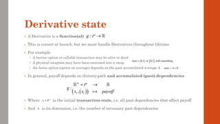
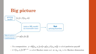
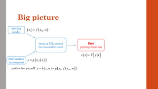


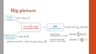
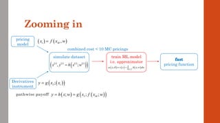


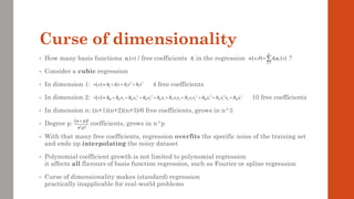
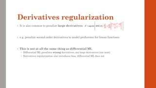
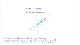
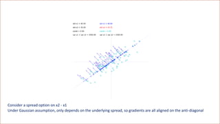
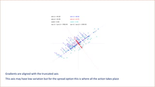
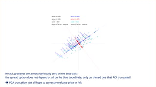
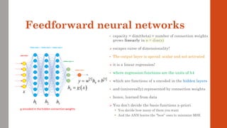
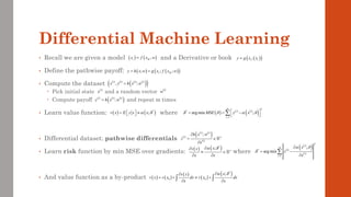
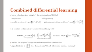
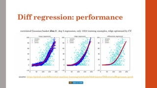
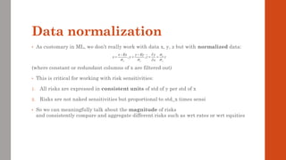
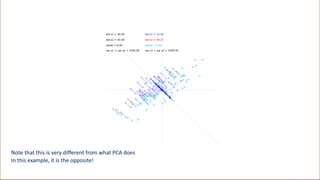
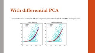
![Example: Gaussian basket
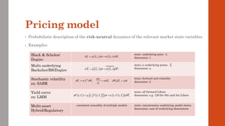
• Black & Scholes is not a representative example
• Because its dimension is 1: x = {spot}
• Most situations in finance are high-dimensional
• e.g. LMM with 3m Libors over 30y: x = {all forward Libors}, dimension = 120
• With netting sets or trading books, dimension generally in the 100s or more
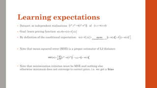
• A more representative example is the basket option in the correlated Bachelier model
Equally simple, with analytic solution
But, crucially, multidimensional x = {spot[1], spot[2], …, spot[n]}
Path generation:
chol: choleski decomp, sigma: covariance matrix and N^(-1) applied elementwise
Cashflow: a: (fixed) weights in the basket and K: strike
Payoff:
Analytic solution: Bach: classic Bachelier formula
( ) ( ) ( )
1
;
T
x f x w x chol N w
−
= = +
( ) ( )
T
T T
g x a x K
+
= −
( ) ( ) ( ) ( )
( )
1
; ; T
h x w g f x w a x chol N w K
+
−
= = + −
( ) ( )
( ) ( )
0,1
, , ; ,
n
T T
v x h x w dw Bach a x a a K T
= =
](https://image.slidesharecdn.com/dlm-masterclass-v2-talk-220319152430/85/Differential-Machine-Learning-Masterclass-49-320.jpg)

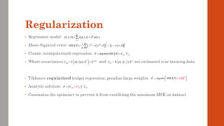


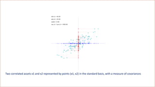

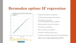


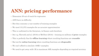


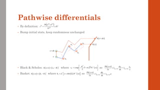


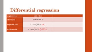
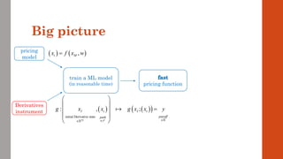
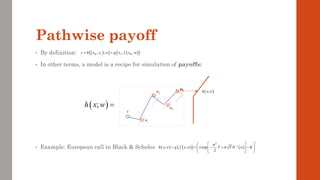
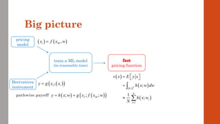
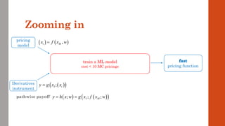
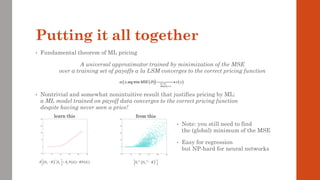
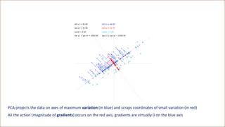
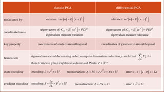
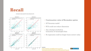
![regression objective solution
standard
regularized
differential
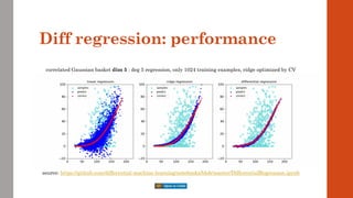
Differential regression
( )
2
*
arg min MSE
=
+
( ) ( )
1
*
arg min
n
j j
j
M E
SE MS
=
=
+
( )
*
arg min MSE
= * 1
y
C C
−
=
( )
1
*
y
K
C I C
−
+
=
1
*
1 1
n n
z
j jj j j
j j
y
C C
C C
−
= =
=
+ +
• Where is the covariance matrix of the derivatives of basis functions wrt x_j
• example: cubic regr. dim 2
• and is the vector of covariances of phi_j with z[j], the j-th pathwise derivative
( ) ( )
T K K
jj j j
C E x x
=
( )
( ) ( )
1
,..., K K
j
j j
x x
x
x x
=
( )
( )
( )
2 2 2 2 3 3
1 2 1 2 1 2 1 2 1 2 1 2 1 2
2 2
1 1 2 1 2 1 2 2 1
2 2
2 1 2 2 1 1 1 2
, [ 1 ]
, [ 0 1 0 2 0 2 3 0 ]
, [ 0 0 1 0 2 2 0 3 ]
x x x x x x x x x x x x x x
x x x x x x x x
x x x x x x x x
=
=
=
( )
z K
j j
C E x z j
=
](https://image.slidesharecdn.com/dlm-masterclass-v2-talk-220319152430/85/Differential-Machine-Learning-Masterclass-99-320.jpg)


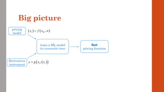
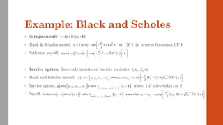
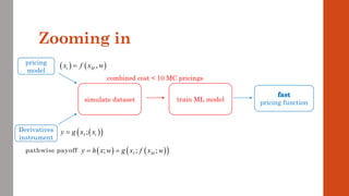
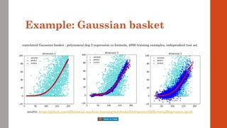
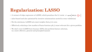
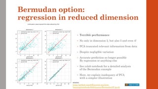
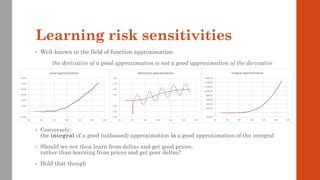
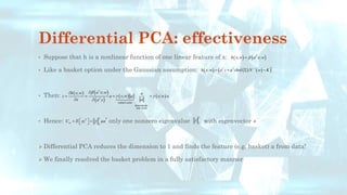
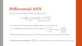
![[Variation = magnitude of data coordinates] is the wrong metric
The correct metric is the magnitude of directional derivatives, called relevance](https://image.slidesharecdn.com/dlm-masterclass-v2-talk-220319152430/85/Differential-Machine-Learning-Masterclass-110-320.jpg)


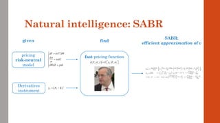
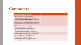
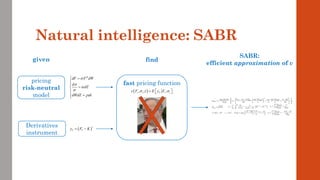
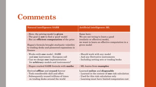
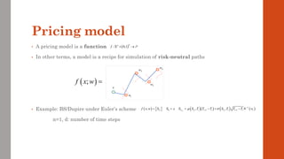
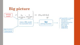
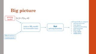
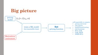
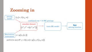
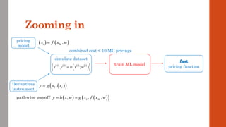
The document reviews the application of machine learning (ML) in derivatives pricing and risk assessment, focusing on both conventional ML methods and differential ML techniques. It emphasizes the importance of efficient computation for pricing models, specifically through the use of exemplary algorithms such as the SABR model, and highlights the potential of ML to significantly reduce computational costs in risk calculations. The document discusses a framework for training ML models to improve speed and efficiency in pricing functions for various derivatives instruments.