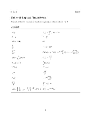
S. Boyd                                                                                               EE102


Table of Laplace Transforms
Remember that we consider all functions (signals) as defined only on t ≥ 0.

General
                                                                 ∞
 f (t)                                    F (s) =                    f (t)e−st dt
                                                             0

 f +g                                     F +G

 αf (α ∈ R)                               αF

 df
                                          sF (s) − f (0)
 dt
 dk f                                                                               df              dk−1 f
                                          sk F (s) − sk−1 f (0) − sk−2                 (0) − · · · − k−1 (0)
 dtk                                                                                dt              dt
                 t                                       F (s)
 g(t) =              f (τ ) dτ            G(s) =
             0                                             s
                                          1
 f (αt), α > 0                              F (s/α)
                                          α
 eat f (t)                                F (s − a)

                                               dF
 tf (t)                                   −
                                               ds
                                                         k
  k                                                 kd   F (s)
 t f (t)                                  (−1)
                                                         dsk
 f (t)                                         ∞
                                                   F (s) ds
   t                                       s

                 0          0≤t<T
 g(t) =                           ,T ≥0   G(s) = e−sT F (s)
                 f (t − T ) t ≥ T


                                               1
Specific

                        1
          1
                        s
          δ             1

          δ (k)         sk

                        1
          t
                        s2
          tk                1
             ,k≥0
          k!            sk+1
                         1
          eat
                        s−a
                             s        1/2    1/2
          cos ωt                  =       +
                        s2   +ω 2   s − jω s + jω
                             ω       1/2j   1/2j
          sin ωt                  =       −
                        s2   +ω 2   s − jω s + jω
                        s cos φ − ω sin φ
          cos(ωt + φ)
                             s2 + ω 2
                            s+a
          e−at cos ωt
                        (s + a)2 + ω 2
                              ω
          e−at sin ωt
                        (s + a)2 + ω 2


                                2
Notes on the derivative formula at t = 0
The formula L(f ) = sF (s) − f (0− ) must be interpreted very carefully when f has a discon-
tinuity at t = 0. We’ll give two examples of the correct interpretation.
    First, suppose that f is the constant 1, and has no discontinuity at t = 0. In other words,
f is the constant function with value 1. Then we have f = 0, and f (0− ) = 1 (since there is
no jump in f at t = 0). Now let’s apply the derivative formula above. We have F (s) = 1/s,
so the formula reads
                                    L(f ) = 0 = sF (s) − 1
which is correct.
    Now, let’s suppose that g is a unit step function, i.e., g(t) = 1 for t > 0, and g(0) = 0.
In contrast to f above, g has a jump at t = 0. In this case, g = δ, and g(0− ) = 0. Now let’s
apply the derivative formula above. We have G(s) = 1/s (exactly the same as F !), so the
formula reads
                                   L(g ) = 1 = sG(s) − 0
which again is correct.
   In these two examples the functions f and g are the same except at t = 0, so they have
the same Laplace transform. In the first case, f has no jump at t = 0, while in the second
case g does. As a result, f has no impulsive term at t = 0, whereas g does. As long as you
keep track of whether your function has, or doesn’t have, a jump at t = 0, and apply the
formula consistently, everything will work out.


                                              3

Laplace table

  • 1.
    S. Boyd EE102 Table of Laplace Transforms Remember that we consider all functions (signals) as defined only on t ≥ 0. General ∞ f (t) F (s) = f (t)e−st dt 0 f +g F +G αf (α ∈ R) αF df sF (s) − f (0) dt dk f df dk−1 f sk F (s) − sk−1 f (0) − sk−2 (0) − · · · − k−1 (0) dtk dt dt t F (s) g(t) = f (τ ) dτ G(s) = 0 s 1 f (αt), α > 0 F (s/α) α eat f (t) F (s − a) dF tf (t) − ds k k kd F (s) t f (t) (−1) dsk f (t) ∞ F (s) ds t s 0 0≤t<T g(t) = ,T ≥0 G(s) = e−sT F (s) f (t − T ) t ≥ T 1
  • 2.
    Specific 1 1 s δ 1 δ (k) sk 1 t s2 tk 1 ,k≥0 k! sk+1 1 eat s−a s 1/2 1/2 cos ωt = + s2 +ω 2 s − jω s + jω ω 1/2j 1/2j sin ωt = − s2 +ω 2 s − jω s + jω s cos φ − ω sin φ cos(ωt + φ) s2 + ω 2 s+a e−at cos ωt (s + a)2 + ω 2 ω e−at sin ωt (s + a)2 + ω 2 2
  • 3.
    Notes on thederivative formula at t = 0 The formula L(f ) = sF (s) − f (0− ) must be interpreted very carefully when f has a discon- tinuity at t = 0. We’ll give two examples of the correct interpretation. First, suppose that f is the constant 1, and has no discontinuity at t = 0. In other words, f is the constant function with value 1. Then we have f = 0, and f (0− ) = 1 (since there is no jump in f at t = 0). Now let’s apply the derivative formula above. We have F (s) = 1/s, so the formula reads L(f ) = 0 = sF (s) − 1 which is correct. Now, let’s suppose that g is a unit step function, i.e., g(t) = 1 for t > 0, and g(0) = 0. In contrast to f above, g has a jump at t = 0. In this case, g = δ, and g(0− ) = 0. Now let’s apply the derivative formula above. We have G(s) = 1/s (exactly the same as F !), so the formula reads L(g ) = 1 = sG(s) − 0 which again is correct. In these two examples the functions f and g are the same except at t = 0, so they have the same Laplace transform. In the first case, f has no jump at t = 0, while in the second case g does. As a result, f has no impulsive term at t = 0, whereas g does. As long as you keep track of whether your function has, or doesn’t have, a jump at t = 0, and apply the formula consistently, everything will work out. 3